Chapter 29 Time-Varying Treatment and Confounding

Studies with time-varying treatments are common in biomedical and social sciences. James Robins championed the research in biostatistics. A classic example is that HIV patients may take azidothymidine, an antiretroviral medication, on and off over time (Robins et al.,, 2000; Hernán et al.,, 2000). Similar problems also exist in other fields. In education, a classic example is that students may receive different types of instructions over time (Hong and Raudenbush,, 2008). In political science, a classic example is that candidates continuously recalibrate their campaign strategy based on time-varying polls and opponent actions (Blackwell,, 2013).

Causal inference with time-varying treatments is not a simple extension of causal inference with a treatment at a single time point. The main challenge is time-varying confounding. Even if we assume all time-varying confounders are observed, we still face statistical challenges in adjusting for those confounders. On the one hand, we should stratify on these confounders to adjust for confounding; on the other hand, stratifying on post-treatment variables will cause bias. Due to these two conflicting goals, causal inference with time-varying treatments and confounding requires more sophisticated statistical methods. It is the main topic of this chapter.

To minimize the notational burden, I will use the setting with treatments at two time points to convey the most important ideas. Extensions to treatments at multiple time points can be conceptually straightforward although technical complexities will arise in finite samples. I will discuss the complexities and relegate general results to Problems 29.7–29.10.

149 Basic setup and sequential ignorability

Start with treatments at two time points. The temporal order (not the causal diagram) of the variables with two time points is below:

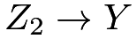
X_{0}\rightarrow Z_{1}\rightarrow X_{1}\rightarrow Z_{2}\rightarrow Y

where

  • •

    X_{0} denotes the baseline pre-treatment covariates;

  • •

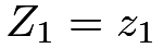
    Z_{1} denotes the treatment at time point 1;

  • •

    X_{1} denotes the time-varying covariates between the treatments at time points 1 and 2;

  • •

    Z_{2} denotes the treatment at time point 2;

  • •

    Y denotes the outcome.

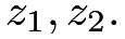
With binary treatments (Z_{1},Z_{2}), each unit has four potential outcomes
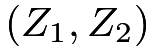

Y(z_{1},z_{2})\text{ for }z_{1},z_{2}=0,1.

The observed outcome equals

Y=Y(Z_{1},Z_{2})=\sum_{z_{1}=0,1}\sum_{z_{2}=0,1}1(Z_{1}=z_{1})1(Z_{2}=z_{2})Y(z_{1},z_{2}).

I will focus on the canonical setting with sequential ignorability, that is, the treatments are sequentially randomized given the observed history.

Assumption 29.1 (sequential ignorability)

(1) Z_{1} is randomized given X_{0}:

Z_{1}\ind Y(z_{1},z_{2})\mid X_{0}\text{ for }z_{1},z_{2}=0,1.

(2) Z_{2} is randomized given (Z_{1},X_{1},X_{0}):

Z_{2}\ind Y(z_{1},z_{2})\mid(Z_{1},X_{1},X_{0})\text{ for }z_{1},z_{2}=0,1.

Figure 46 is a simple causal diagram corresponding to Assumption 29.1, which does not contain any unmeasured confounding.

\textstyle{Z_{1}\ignorespaces\ignorespaces\ignorespaces\ignorespaces\ignorespaces\ignorespaces\ignorespaces\ignorespaces\ignorespaces\ignorespaces\ignorespaces\ignorespaces\ignorespaces\ignorespaces}\textstyle{X_{1}\ignorespaces\ignorespaces\ignorespaces\ignorespaces\ignorespaces\ignorespaces\ignorespaces\ignorespaces\ignorespaces}\textstyle{Z_{2}\ignorespaces\ignorespaces\ignorespaces\ignorespaces}\textstyle{Y}
Figure 46: Assumption 29.1 holds without unmeasured confounding U between X_{1} and Y. The causal diagram conditions on the pre-treatment covariates X_{0}.

Figure 47 is a more complex causal diagram corresponding to Assumption 29.1. Sequential ignorability rules out only the confounding between the treatment (Z_{1},Z_{2}) and the outcome Y, but allows for unmeasured confounding between the time-varying covariate X_{1} and the outcome Y. The possible existence of U causes many subtle issues even under sequential ignorability.

\textstyle{Z_{1}\ignorespaces\ignorespaces\ignorespaces\ignorespaces\ignorespaces\ignorespaces\ignorespaces\ignorespaces\ignorespaces\ignorespaces\ignorespaces\ignorespaces\ignorespaces\ignorespaces}\textstyle{X_{1}\ignorespaces\ignorespaces\ignorespaces\ignorespaces\ignorespaces\ignorespaces\ignorespaces\ignorespaces\ignorespaces}\textstyle{Z_{2}\ignorespaces\ignorespaces\ignorespaces\ignorespaces}\textstyle{Y}\textstyle{U\ignorespaces\ignorespaces\ignorespaces\ignorespaces\ignorespaces\ignorespaces\ignorespaces\ignorespaces}
Figure 47: Assumption 29.1 holds with unmeasured confounding between X_{1} and Y. The causal diagram conditions on the pre-treatment covariates X_{0}.

150 g-formula and outcome modeling

Recall the outcome-based identification formula with a treatment at a single time point:

E\{Y(z)\}=E\{E(Y\mid Z=z,X)\}.

With discrete X, it reduces to

E\{Y(z)\}=\sum_{x}E(Y\mid Z=z,X=x)\textup{pr}(X=x);

with continuous X, it reduces to

E\{Y(z)\}=\int E(Y\mid Z=z,X=x)f(x)\text{d}x.

The following result extends it to the setting with treatments at two time points.

Theorem 29.1

Under Assumption 29.1,

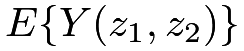
E\{Y(z_{1},z_{2})\}=E\Big[E\{E(Y\mid z_{2},z_{1},X_{1},X_{0})\mid z_{1},X_{0}\}\Big]. (139)

In Theorem 29.1, I simplify the notation ‘Z_{2}=z_{2}” to “z_{2}”. To void complex formulas in this chapter, I will use the lowercase letter to represent the event that the random variable takes the corresponding value. With discrete X_{0} and X_{1}, the identification formula (139) reduces to

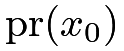
E\{Y(z_{1},z_{2})\}=\sum_{x_{0}}\sum_{x_{1}}E(Y\mid z_{2},z_{1},x_{1},x_{0})\textup{pr}(x_{1}\mid z_{1},x_{0})\textup{pr}(x_{0}); (140)

with continuous X_{0} and X_{1}, the identification formula (139) reduces to

E\{Y(z_{1},z_{2})\}=\int\int E(Y\mid z_{2},z_{1},x_{1},x_{0})f(x_{1}\mid z_{1},x_{0})f(x_{0})\text{d}x_{1}\text{d}x_{0}. (141)

Compare (140) with the formula based on the law of total probability to gain more insights:

\displaystyle E(Y) \displaystyle= \displaystyle\sum_{x_{0}}\sum_{z_{1}}\sum_{x_{1}}\sum_{z_{2}}E(Y\mid z_{2},z_{1},x_{1},x_{0}) (142)
\displaystyle\qquad\textup{pr}(z_{2}\mid z_{1},x_{1},x_{0})\textup{pr}(x_{1}\mid z_{1},x_{0})\textup{pr}(z_{1}\mid x_{0})\textup{pr}(x_{0}).

Erasing the probabilities of Z_{2} and Z_{1} in (142), we can obtain the formula (141). This is intuitive because the potential outcome Y(z_{1},z_{2}) has the meaning of fixing Z_{1} and Z_{2} at z_{1} and z_{2}, respectively.
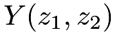
Robins called (140) and (141) the g-formulas. Now I will prove Theorem 29.1.

Proof of Theorem 29.1: By the tower property,

E\{Y(z_{1},z_{2})\}=E\Big[E\{Y(z_{1},z_{2})\mid X_{0}\}\Big],

so I will focus on E\{Y(z_{1},z_{2})\mid X_{0}\}. By Assumption 29.1(1) and the tower property,

\displaystyle E\{Y(z_{1},z_{2})\mid X_{0}\} \displaystyle= \displaystyle E\{Y(z_{1},z_{2})\mid z_{1},X_{0}\}
\displaystyle= \displaystyle E\Big[E\{Y(z_{1},z_{2})\mid z_{1},X_{1},X_{0}\}\mid z_{1},X_{0}\Big].

By Assumption 29.1(2),

\displaystyle E\{Y(z_{1},z_{2})\mid X_{0}\} \displaystyle= \displaystyle E\Big[E\{Y(z_{1},z_{2})\mid z_{2},z_{1},X_{1},X_{0}\}\mid z_{1},X_{0}\Big]
\displaystyle= \displaystyle E\Big[E\{Y\mid z_{2},z_{1},X_{1},X_{0}\}\mid z_{1},X_{0}\Big].

The formula (139) follows. \square

150.1 Plug-in estimation based on outcome modeling

The g-formulas (140) and (141) suggest that to estimate the means of the potential outcomes, we need to model E(Y\mid z_{2},z_{1},x_{1},x_{0}), \textup{pr}(x_{1}\mid z_{1},x_{0}) and \textup{pr}(x_{0}). With these fitted models, we can plug them into the g-formulas.

With some special functional forms, this task can be simplified. Example 29.1 below gives the results under a linear model for the outcome.

Example 29.1

Assume a linear outcome model

E(Y\mid z_{2},z_{1},x_{1},x_{0})=\beta_{0}+\beta_{1}z_{2}+\beta_{2}z_{1}+\beta_{3}x_{1}+\beta_{4}x_{0}.

We can verify that

\displaystyle E\{Y(z_{1},z_{2})\} \displaystyle= \displaystyle\sum_{x_{0}}\sum_{x_{1}}(\beta_{0}+\beta_{1}z_{2}+\beta_{2}z_{1}+\beta_{3}x_{1}+\beta_{4}x_{0})\textup{pr}(x_{1}\mid z_{1},x_{0})\textup{pr}(x_{0})
\displaystyle= \displaystyle\beta_{0}+\beta_{1}z_{2}+\beta_{2}z_{1}+\beta_{3}\sum_{x_{0}}E(X_{1}\mid z_{1},x_{0})\textup{pr}(x_{0})+\beta_{4}E(X_{0}).

Define

E\{X_{1}(z_{1})\}=\sum_{x_{0}}E(X_{1}\mid z_{1},x_{0})\textup{pr}(x_{0}) (143)

to simplify the formula as

E\{Y(z_{1},z_{2})\}=\beta_{0}+\beta_{1}z_{2}+\beta_{2}z_{1}+\beta_{3}E\{X_{1}(z_{1})\}+\beta_{4}E(X_{0}).

In (143), I introduce the potential outcome of X_{1} under the treatment Z_{1}=z_{1} at time point 1. It is reasonable because the right-hand side of (143) is the identification formula of E\{X_{1}(z_{1})\} under ignorability X_{1}(z_{1})\ind Z_{1}\mid X_{0} for z_{1}=0,1. We do not really need the potential outcome X_{1}(z_{1}) and the ignorability, but it is a convenient notation and matches our previous discussion.
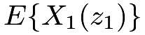
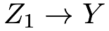
Define \tau_{Z_{1}\rightarrow X_{1}}=E\{X_{1}(1)-X_{1}(0)\}. We can verify that

\displaystyle E\{Y(1,0)-Y(0,0)\} \displaystyle= \displaystyle\beta_{2}+\beta_{3}\tau_{Z_{1}\rightarrow X_{1}},
\displaystyle E\{Y(0,1)-Y(0,0)\} \displaystyle= \displaystyle\beta_{1},
\displaystyle E\{Y(1,1)-Y(0,0)\} \displaystyle= \displaystyle\beta_{1}+\beta_{2}+\beta_{3}\tau_{Z_{1}\rightarrow X_{1}}.

Therefore, we can estimate the effect of (Z_{1},Z_{2}) on Y based on the above formulas by first estimating the regression coefficients \betas and the average causal effect of Z_{1} on X_{1} using standard methods.

If we further assume a linear model for X_{1}

E(X_{1}\mid Z_{1},X_{0})=\gamma_{0}+\gamma_{1}z_{1}+\gamma_{2}x_{0},

then \tau_{Z_{1}\rightarrow X_{1}}=\gamma_{1} and

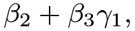
\displaystyle E\{Y(1,0)-Y(0,0)\} \displaystyle= \displaystyle\beta_{2}+\beta_{3}\gamma_{1}, (144)
\displaystyle E\{Y(0,1)-Y(0,0)\} \displaystyle= \displaystyle\beta_{1}, (145)
\displaystyle E\{Y(1,1)-Y(0,0)\} \displaystyle= \displaystyle\beta_{1}+\beta_{2}+\beta_{3}\gamma_{1}. (146)

The formulas in (144)–(146) are intuitive based on Figure 48 with regression coefficients on the arrows. In (144), the effect of Z_{1} equals the sum of the coefficients on the paths Z_{1}\rightarrow Y and Z_{1}\rightarrow X_{1}\rightarrow Y; in (145), the effect of Z_{2} equals the coefficient on the path Z_{2}\rightarrow Y; in (146), the total effect of (Z_{1},Z_{2}) equals the sum of the coefficients on the paths Z_{1}\rightarrow Y, Z_{1}\rightarrow X_{1}\rightarrow Y and Z_{2}\rightarrow Y.
\textstyle{Z_{1}\ignorespaces\ignorespaces\ignorespaces\ignorespaces\ignorespaces\ignorespaces\ignorespaces\ignorespaces\ignorespaces\ignorespaces\ignorespaces\ignorespaces\ignorespaces\ignorespaces}\scriptstyle{\gamma_{1}}\scriptstyle{\beta_{2}}\textstyle{X_{1}\ignorespaces\ignorespaces\ignorespaces\ignorespaces\ignorespaces\ignorespaces\ignorespaces\ignorespaces\ignorespaces}\scriptstyle{\beta_{3}}\textstyle{Z_{2}\ignorespaces\ignorespaces\ignorespaces\ignorespaces}\scriptstyle{\beta_{1}}\textstyle{Y}
Figure 48: A linear causal diagram with coefficients on the arrows, conditional on the pre-treatment covariates X_{0}.

However, Robins and Wasserman, (1997) pointed out a surprising drawback of the plug-in estimation based on outcome modeling. They showed that with model misspecification in this strategy, data analyzers may falsely reject the null hypothesis of zero causal effect of (Z_{1},Z_{2}) on Y even when the true effect is zero in the data-generating process. They called it the g-null paradox. Perhaps surprisingly, they show that the g-null paradox may even arise in the simple linear outcome model in Example 29.1. McGrath et al., (2021) revisited this paradox. See Problem 29.1 for more details.

150.2 Recursive estimation based on outcome modeling

The plug-in estimation in Section 150.1 involves modeling the time-varying confounder X_{1} and causes the unpleasant g-null paradox. It is not a desirable method.

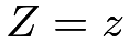
Recall the outcome regression estimator with a treatment at a single time based on E\{Y(z)\}=E\{E(Y\mid Z=z,X)\}. We first fit a model of Y on X using the subset of the data with Z=z, and obtain the fitted values \hat{Y}_{i}(z) for all units. We then obtain the estimator

\hat{E}\{Y(z)\}=n^{-1}\sum_{i=1}^{n}\hat{Y}_{i}(z).

Similarly, the recursive expectation formula in (139) motivates a simpler method for estimation. Start from the inner conditional expectation, denoted by

\tilde{Y}_{2}(z_{1},z_{2})=E(Y\mid Z_{2}=z_{2},Z_{1}=z_{1},X_{1},X_{0}).

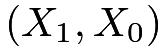
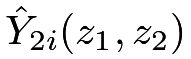
We can fit a model of Y on (X_{1},X_{0}) using the subset of the data with (Z_{2}=z_{2},Z_{1}=z_{1}), and obtain the fitted values \hat{Y}_{2i}(z_{1},z_{2}) for all units. Move on to outer conditional expectation, denoted by

\tilde{Y}_{1}(z_{1},z_{2})=E\{\tilde{Y}_{2}(z_{1},z_{2})\mid Z_{1}=z_{1},X_{0}\}.

We can fit a model of \hat{Y}_{2}(z_{1},z_{2}) on X_{0} using the subset of data with Z_{1}=z_{1}, and obtain the fitted values \hat{Y}_{1i}(z_{1},z_{2}) for all units. The final estimator for E\{Y(z_{1},z_{2})\} is then

\hat{E}\{Y(z_{1},z_{2})\}=n^{-1}\sum_{i=1}^{n}\hat{Y}_{1i}(z_{1},z_{2}).

The above recursive estimation does not involve fitting a model for X_{1} and avoids the g-null paradox. See Problem 29.2 for a special case. However, the estimator based on recursive regression is not easy to implement because it involves modeling variables that do not correspond to the natural structure of the causal diagram, e.g., \tilde{Y}_{2}(z_{1},z_{2}).

151 Inverse propensity score weighting

Recall the IPW identification formula with a treatment at a single time point:

E\{Y(z)\}=E\left\{\frac{1(Z=z)Y}{\textup{pr}(Z=z\mid X)}\right\}.

The following result extends it to the setting with a treatment at two time points. Define

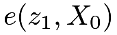
e(z_{1},X_{0})=\textup{pr}(Z_{1}=z_{1}\mid X_{0})

and

e(z_{2},Z_{1},X_{1},X_{0})=\textup{pr}(Z_{2}=z_{2}\mid Z_{1},X_{1},X_{0})

as the propensity scores at time points 1 and 2, respectively.

Theorem 29.2

Under Assumption 29.1,

E\{Y(z_{1},z_{2})\}=E\left\{\frac{1(Z_{1}=z_{1})1(Z_{2}=z_{2})Y}{e(z_{1},X_{0})e(z_{2},Z_{1},X_{1},X_{0})}\right\}. (147)

Theorem 29.2 reveals the omitted overlap assumption:

0<e(z_{1},X_{0})<1,\quad 0<e(z_{2},Z_{1},X_{1},X_{0})<1

for all z_{1} and z_{2}. If some propensity scores are 0 or 1, then the identification formula (147) blows up to infinity.

Proof of Theorem 29.2: Conditioning on (Z_{1},X_{1},X_{0}) and using Assumption 29.1(2), we can simplify the right-hand side of (147) as

\displaystyle E\left\{\frac{1(Z_{1}=z_{1})1(Z_{2}=z_{2})Y(z_{1},z_{2})}{\textup{pr}(Z_{1}=z_{1}\mid X_{0})\textup{pr}(Z_{2}=z_{2}\mid Z_{1},X_{1},X_{0})}\right\} (148)
\displaystyle= \displaystyle E\left\{\frac{1(Z_{1}=z_{1})\textup{pr}(Z_{2}=z_{2}\mid Z_{1},X_{1},X_{0})E(Y(z_{1},z_{2})\mid Z_{1},X_{1},X_{0})}{\textup{pr}(Z_{1}=z_{1}\mid X_{0})\textup{pr}(Z_{2}=z_{2}\mid Z_{1},X_{1},X_{0})}\right\}
\displaystyle= \displaystyle E\left\{\frac{1(Z_{1}=z_{1})}{\textup{pr}(Z_{1}=z_{1}\mid X_{0})}E(Y(z_{1},z_{2})\mid Z_{1},X_{1},X_{0})\right\}
\displaystyle= \displaystyle E\left\{\frac{1(Z_{1}=z_{1})}{\textup{pr}(Z_{1}=z_{1}\mid X_{0})}Y(z_{1},z_{2})\right\},

where (148) follows from the tower property.

Conditioning on X_{0} and using Assumption 29.1(1), we can simplify the right-hand side of (148) as

\displaystyle E\left\{\frac{\textup{pr}(Z_{1}=z_{1}\mid X_{0})}{\textup{pr}(Z_{1}=z_{1}\mid X_{0})}E(Y(z_{1},z_{2})\mid X_{0})\right\}
\displaystyle= \displaystyle E\left\{E(Y(z_{1},z_{2})\mid X_{0})\right\}
\displaystyle= \displaystyle E\{Y(z_{1},z_{2})\},

where, again, the last line follows from the tower property. \square

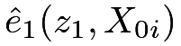
The estimator based on IPW is much simpler which only involves modeling two binary treatment indicators. First, we can fit a model of Z_{1} on X_{0} to obtain the fitted values \hat{e}_{1}(z_{1},X_{0i}) and fit a model of Z_{2} on (Z_{1},X_{1},X_{0}) to obtain the fitted values \hat{e}_{2}(z_{2},Z_{1i},X_{1i},X_{0i}) for all units. Then, we obtain the following IPW estimator:

\hat{E}^{\textup{ht}}\{Y(z_{1},z_{2})\}=n^{-1}\sum_{i=1}^{n}\frac{1(Z_{1i}=z_{1})1(Z_{2i}=z_{2})Y_{i}}{\hat{e}_{1}(z_{1},X_{0i})\hat{e}_{2}(z_{2},Z_{1i},X_{1i},X_{0i})}.

Similar to the discussion in Chapter 11, the HT estimator is not invariant to the location shift of the outcome and suffers from instability in finite samples. A modified Hajek-type estimator is \hat{E}^{\textup{haj}}\{Y(z_{1},z_{2})\}=\hat{E}^{\textup{ht}}\{Y(z_{1},z_{2})\}/\hat{1}^{\textup{ht}}(z_{1},z_{2}), where

\hat{1}^{\textup{ht}}(z_{1},z_{2})=n^{-1}\sum_{i=1}^{n}\frac{1(Z_{1i}=z_{1})1(Z_{2i}=z_{2})}{\hat{e}_{1}(z_{1},X_{0i})\hat{e}_{2}(z_{2},Z_{1i},X_{1i},X_{0i})}.

152 Multiple time points

Extending the estimation strategies in Sections 150 and 151 is not immediate with multiple time points. Even with a binary treatment and K time points, the number of treatment combinations grows exponentially with K (for example, 2^{5}=32 and 2^{10}=1024). Consequently, the outcome regression and IPW estimators in Sections 150 and 151 are not feasible in finite samples because they require enough data for every combination of the treatment levels.

152.1 Marginal structural model

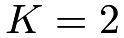
A powerful approach is based on the marginal structural model (MSM) (Robins et al.,, 2000; Hernán et al.,, 2000). For simplicity of notation, I will only present the MSM with K=2 although its main use is in the general case.
Definition 29.1 (MSM)

The marginal mean of Y(z_{1},z_{2}) equals

E\{Y(z_{1},z_{2})\}=f(z_{1},z_{2};\beta).

A leading example of Definition 29.1 is E\{Y(z_{1},z_{2})\}=\beta_{0}+\beta_{1}z_{1}+\beta_{2}z_{2}. It is also straightforward to include the baseline covariates in the model. Definition 29.2 below extends Definition 29.1.

Definition 29.2 (MSM with baseline covariates)

The mean of Y(z_{1},z_{2}) conditional on X_{0} equals

E\{Y(z_{1},z_{2})\mid X_{0}\}=f(z_{1},z_{2},X_{0};\beta).

A leading example of Definition 29.2 is

E\{Y(z_{1},z_{2})\mid X_{0}\}=\beta_{0}+\beta_{1}z_{1}+\beta_{2}z_{2}+\beta_{3}^{\mkern-1.5mu\mathsf{T}}X_{0}. (149)

If we observe all the potential outcomes, we can solve \beta from the following minimization problem:

\beta=\arg\min_{b}\sum_{z_{2}}\sum_{z_{1}}E\{Y(z_{1},z_{2})-f(z_{1},z_{2},X_{0};b)\}^{2}. (150)

For simplicity, I focus on the least squares formulation. We can also extend the discussion to general models; see Problem 29.4 for an example of the logistic model.

Under sequential ignorability, we can solve \beta from the following minimization problem that only involves observables.

Theorem 29.3 (IPW under MSM)

Under Assumption 29.1 and Definition 29.2, the \beta in (150) equals

\beta=\arg\min_{b}\sum_{z_{2}}\sum_{z_{1}}E\left[\frac{1(Z_{1}=z_{1})1(Z_{2}=z_{2})}{e(z_{1},X_{0})e(z_{2},Z_{1},X_{1},X_{0})}\{Y-f(z_{1},z_{2},X_{0};b)\}^{2}\right].

The proof of Theorem 29.3 is similar to that of Theorem 29.2. I relegate it to Problem 29.3.

Theorem 29.3 implies a simple estimation strategy based on weighted regressions. For instance, under (149), we can fit WLS of Y_{i} on (1,Z_{1i},Z_{2i},X_{0i}) with weights \hat{e}_{1}^{-1}(Z_{1i},X_{0i})\hat{e}_{2i}^{-1}(Z_{2i},Z_{i1},X_{1i},X_{0i}).

152.2 Structural nested model

A key problem of IPW is that it is not applicable if the overlap assumption is violated. To address this challenge, Robins proposed the structural nested model. Again, to simplify the presentation, I only review the version with two time points.

Definition 29.3 (structural nested model)

The conditional effect at time point 1 is

E\{Y(z_{1},0)-Y(0,0)\mid Z_{1}=z_{1},X_{0}\}=g_{1}(z_{1},X_{0};\beta)

for all z_{1}, and the conditional effect at time point 2 is

E\{Y(z_{1},z_{2})-Y(z_{1},0)\mid Z_{2}=z_{2},Z_{2}=z_{1},X_{1},X_{0}\}=g_{2}(z_{2},z_{1},X_{1},X_{0};\beta)

for all z_{1},z_{2}.

In Definition 29.3, two logical restrictions are

g_{1}(0,X_{0};\beta)=0

and

g_{2}(0,z_{1},X_{1},X_{0};\beta)=0\text{ for all }z_{1}.

Two leading choices of Definition 29.3 are below.

Example 29.2

Assume

\begin{cases}g_{1}(z_{1},X_{0};\beta)=\beta_{1}z_{1},\\
g_{2}(z_{2},z_{1},X_{1},X_{0};\beta)=(\beta_{2}+\beta_{3}z_{1})z_{2}.\end{cases}
Example 29.3

Assume

\begin{cases}g_{1}(z_{1},X_{0};\beta)=(\beta_{1}+\beta_{2}^{\mkern-1.5mu\mathsf{T}}X_{0})z_{1},\\
g_{2}(z_{2},z_{1},X_{1},X_{0};\beta)=(\beta_{3}+\beta_{4}z_{1}+\beta_{5}^{\mkern-1.5mu\mathsf{T}}X_{1})z_{2}.\end{cases}

Compare Definitions 29.2 and 29.3. The structural nested model allows for adjusting for the baseline covariates as well as the time-varying covariates whereas the marginal structural model only allows for adjusting for the baseline covariates. The estimation under Definition 29.3 is more involved. A strategy is to estimate the parameter based on estimating equations.

I first introduce two important building blocks for discussing the estimation. Define

U_{2}(\beta)=Y-g_{2}(Z_{2},Z_{1},X_{1},X_{0};\beta)

and

U_{1}(\beta)=Y-g_{2}(Z_{2},Z_{1},X_{1},X_{0};\beta)-g_{1}(Z_{1},X_{0};\beta).

They are not directly computable from the data because they depend on the true value of the parameter \beta. At the true value, they have the following properties.

Lemma 29.1

Under Assumption 29.1 and Definition 29.3, we have

\displaystyle E\{U_{2}(\beta)\mid Z_{2},Z_{1},X_{1},X_{0}\} \displaystyle= \displaystyle E\{U_{2}(\beta)\mid Z_{1},X_{1},X_{0}\}
\displaystyle= \displaystyle E\{Y(Z_{1},0)\mid Z_{1},X_{1},X_{0}\}

and

\displaystyle E\{U_{1}(\beta)\mid Z_{1},X_{0}\} \displaystyle= \displaystyle E\{U_{1}(\beta)\mid X_{0}\}
\displaystyle= \displaystyle E\{Y(0,0)\mid X_{0}\}.

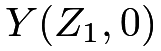
Lemma 29.1 involves a subtle notation Y(Z_{1},0) because Z_{1} is random. It should be read as Y(Z_{1},0)=Z_{1}Y(1,0)+(1-Z_{1})Y(0,0). Based on the definitions and Lemma 29.1, U_{1}(\beta) acts as the control potential outcome before receiving any treatment and U_{2}(\beta) acts as the control potential outcome after receiving the treatment at time point 1.

Proof of Lemma 29.1: Part 1. We have

\displaystyle E\{U_{2}(\beta)\mid Z_{2}=1,Z_{1},X_{1},X_{0}\}
\displaystyle= \displaystyle E\{Y(Z_{1},1)-g_{2}(1,Z_{1},X_{1},X_{0};\beta)\mid Z_{2}=1,Z_{1},X_{1},X_{0}\}
\displaystyle= \displaystyle E\{Y(Z_{1},0)\mid Z_{2}=1,Z_{1},X_{1},X_{0}\}

and

\displaystyle E\{U_{2}(\beta)\mid Z_{2}=0,Z_{1},X_{1},X_{0}\}
\displaystyle= \displaystyle E\{Y(Z_{1},0)-g_{2}(0,Z_{1},X_{1},X_{0};\beta)\mid Z_{2}=0,Z_{1},X_{1},X_{0}\}
\displaystyle= \displaystyle E\{Y(Z_{1},0)\mid Z_{2}=0,Z_{1},X_{1},X_{0}\}

so

\displaystyle E\{U_{2}(\beta)\mid Z_{2},Z_{1},X_{1},X_{0}\} \displaystyle= \displaystyle E\{Y(Z_{1},0)\mid Z_{2},Z_{1},X_{1},X_{0}\}
\displaystyle= \displaystyle E\{Y(Z_{1},0)\mid Z_{1},X_{1},X_{0}\}

where the last identity follows from sequential ignorability. Since the last term does not depend on Z_{2}, we also have

E\{U_{2}(\beta)\mid Z_{2},Z_{1},X_{1},X_{0}\}=E\{U_{2}(\beta)\mid Z_{1},X_{1},X_{0}\}.

Part 2. Using the above results, we have

\displaystyle E\{U_{1}(\beta)\mid Z_{1},X_{0}\}
\displaystyle= \displaystyle E\{U_{2}(\beta)-g_{1}(Z_{1},X_{0};\beta)\mid Z_{1},X_{0}\}\qquad(\text{Definition }\ref{def::snm})
\displaystyle= \displaystyle E\left[E\{U_{2}(\beta)-g_{1}(Z_{1},X_{0};\beta)\mid X_{1},Z_{1},X_{0}\}\mid Z_{1},X_{0}\right]\qquad(\text{tower property})
\displaystyle= \displaystyle E\left[E\{Y(Z_{1},0)-g_{1}(Z_{1},X_{0};\beta)\mid X_{1},Z_{1},X_{0}\}\mid Z_{1},X_{0}\right]\qquad(\text{part 1})
\displaystyle= \displaystyle E\{Y(Z_{1},0)-g_{1}(Z_{1},X_{0};\beta)\mid Z_{1},X_{0}\}\qquad(\text{tower property})
\displaystyle= \displaystyle E\{Y(0,0)\mid Z_{1},X_{0}\}\qquad(\text{Definition }\ref{def::snm})
\displaystyle= \displaystyle E\{Y(0,0)\mid X_{0}\}\qquad(\text{sequential ignorability}).

Since the last term does not depend on Z_{1}, we also have

E\{U_{1}(\beta)\mid Z_{1},X_{0}\}=E\{U_{1}(\beta)\mid X_{0}\}.

\square

With Lemma 29.1, we can prove Theorem 29.4 below.

Theorem 29.4

Under Assumption 29.1 and Definition 29.3,

E\Big[h_{2}(Z_{1},X_{1},X_{0})\{Z_{2}-e(1,Z_{1},X_{1},X_{0})\}U_{2}(\beta)\Big]=0

and

E\Big[h_{1}(X_{0})\{Z_{1}-e(1,X_{0})\}U_{1}(\beta)\Big]=0.

for any functions h_{1} and h_{2}, provided that the moments exist.

Proof of Theorem 29.2: Use the tower property by conditioning on (Z_{2},Z_{1},X_{1},X_{0}) and Lemma 29.1 to obtain

\displaystyle E\left[h_{2}(Z_{1},X_{1},X_{0})\{Z_{2}-e(1,Z_{1},X_{1},X_{0})\}E\{U_{2}(\beta)\mid Z_{2},Z_{1},X_{1},X_{0}\}\right]
\displaystyle= \displaystyle E\left[h_{2}(Z_{1},X_{1},X_{0})\{Z_{2}-e(1,Z_{1},X_{1},X_{0})\}E\{U_{2}(\beta)\mid Z_{1},X_{1},X_{0}\}\right].

Use the tower property by conditioning on (Z_{1},X_{1},X_{0}) to show that the last identity equals 0 because E\{Z_{2}-e(1,Z_{1},X_{1},X_{0})\mid Z_{1},X_{1},X_{0}\}=0.

Similarly, use the tower property by conditioning on (Z_{1},X_{0}) and Lemma 29.1 to obtain

\displaystyle E\left[h_{1}(X_{0})\{Z_{1}-e(1,X_{0})\}E\{U_{1}(\beta)\mid Z_{1},X_{0}\}\right]
\displaystyle= \displaystyle E\left[h_{1}(X_{0})\{Z_{1}-e(1,X_{0})\}E\{U_{1}(\beta)\mid X_{0}\}\right].

Use the tower property by conditioning on X_{0} to show that the last identity equals 0 because E\{Z_{1}-e(1,X_{0})\mid X_{0}\}=0. \square

To use Theorem 29.4, we must specify h_{1} and h_{2} to ensure that there are enough equations for solving \beta. Example 29.4 below revisits Example 29.2.

Example 29.4

Under Example 29.2, we can choose h_{1}=1 and h_{2}=(1,Z_{1}) to obtain

\displaystyle E\left[\{Z_{2}-e(1,Z_{1},X_{1},X_{0})\}\{Y-(\beta_{2}+\beta_{3}Z_{1})Z_{2}\}\right] \displaystyle= \displaystyle 0,
\displaystyle E\left[Z_{1}\{Z_{2}-e(1,Z_{1},X_{1},X_{0})\}\{Y-(\beta_{2}+\beta_{3}Z_{1})Z_{2}\}\right] \displaystyle= \displaystyle 0,
\displaystyle E\left[\{Z_{1}-e(1,X_{0})\}\{Y-(\beta_{2}+\beta_{3}Z_{1})Z_{2}-\beta_{1}Z_{1}\}\right] \displaystyle= \displaystyle 0.

We can then solve for the \beta’s from the above linear equations; see Problem 29.6. A natural question is whether alternative choices of (h_{1},h_{2}) can lead to more efficient estimators. The answer is yes. For example, we can choose many (h_{1},h_{2}) and use the generalized method of moment (Hansen,, 1982). The technical details are beyond this book.

Naimi et al., (2017) and Vansteelandt and Joffe, (2014) provided tutorials on the structural nested models.

153 Homework problems

29.1 g-null paradox

Consider the simple causal diagram in Figure 49 without pre-treatment covariates X_{0} and without the arrows from (Z_{1},Z_{2}) to Y. So the effect of (Z_{1},Z_{2}) on Y is zero.

\textstyle{Z_{1}\ignorespaces\ignorespaces\ignorespaces\ignorespaces}\textstyle{X_{1}\ignorespaces\ignorespaces\ignorespaces\ignorespaces}\textstyle{Z_{2}}\textstyle{Y}\textstyle{U\ignorespaces\ignorespaces\ignorespaces\ignorespaces\ignorespaces\ignorespaces\ignorespaces\ignorespaces}
Figure 49: With unmeasured confounding between X_{1} and Y. The causal diagram ignores the pre-treatment covariates X_{0}.

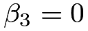
Revisit Example 29.1. Show that the expectation E\{Y(z_{1},z_{2})\} does not depend on (z_{1},z_{2}) if

\beta_{1}=\beta_{2}=0\text{ and }\beta_{3}=0

or

\beta_{1}=\beta_{2}=0\text{ and }E\{X_{1}(z_{1})\}\text{ does not depend on }z_{1}.

holds.

Remark: However, \beta_{3}=0 in the first condition rules out the dependence of Y on X_{1}, contradicting the existence of unmeasured confounder U between X_{1} and Y; the independence of E\{X_{1}(z_{1})\} on z_{1} rules out the dependence of X_{1} on Z_{1}, contradicting with the existence of the arrow from Z_{1} on X_{1}. That is, if there is an unmeasured confounder U between X_{1} and Y and there is an arrow from Z_{1} on X_{1}, then the formula of E\{Y(z_{1},z_{2})\} in Example 29.1 must depend on (z_{1},z_{2}), which leads to a contradiction with the absence of arrows from (Z_{1},Z_{2}) to Y.

29.2 Recursive estimation under the null model

Consider the recursive estimation method in 150.2 under the causal diagram in Problem 29.1. Show that based on linear models, the estimator converges to 0.

29.3 IPW under MSM

Prove Theorem 29.3.

29.4 A nonlinear example of Definition 29.2

Another leading example of Definition 29.2 is

\text{logit}\left[\textup{pr}\{Y(z_{1},z_{2})=1\mid X_{0}\}\right]=\beta_{0}+\beta_{1}z_{1}+\beta_{2}z_{2}+\beta_{3}^{\mkern-1.5mu\mathsf{T}}X_{0}. (151)

If we observe all potential outcomes, we can solve \beta by minimizing the expectation of the negative log-likelihood function (see Chapter 31.F.2 for a simpler version):

\beta=\arg\min_{b}\sum_{z_{2}}\sum_{z_{1}}E\left\{\log(1+e^{\ell})-Y(z_{1},z_{2})\ell\right\} (152)

where \ell=\beta_{0}+\beta_{1}z_{1}+\beta_{2}z_{2}+\beta_{3}^{\mkern-1.5mu\mathsf{T}}X_{0}. Under sequential ignorability, we can solve \beta from the following minimization problem that only involves observables.

Theorem 29.5 (IPW under MSM)

Under Assumption 29.1 and Definition 29.2, the \beta in (152) equals

\beta=\arg\min_{b}\sum_{z_{2}}\sum_{z_{1}}E\left[\frac{1(Z_{1}=z_{1})1(Z_{2}=z_{2})}{e(z_{1},X_{0})e(z_{2},Z_{1},X_{1},X_{0})}\left\{\log(1+e^{\ell})-Y(z_{1},z_{2})\ell\right\}\right].

Prove Theorem 29.5.

Remark: Theorem 29.5 implies a simple estimation strategy based on weighted regressions. For instance, under (151), we can fit weighted logistic regression of Y_{i} on (1,Z_{1i},Z_{2i},X_{0i}) with weights \hat{e}_{1}^{-1}(Z_{1i},X_{0i})\hat{e}_{2i}^{-1}(Z_{2i},Z_{i1},X_{1i},X_{0i}).

29.5 Structural nested model with a single time point

Recall the standard setting of observational studies with IID data drawn from \{X,Z,Y(1),Y(0)\}. Define the propensity score as e(X)=\textup{pr}(Z=1\mid X). Assume

Z\ind Y(0)\mid X

and the following structural nested model.

Definition 29.4 (structural nested model with a single time point)

The conditional mean of the individual effect is

E\{Y(z)-Y(0)\mid Z=z,X\}=g(z,X;\beta).

In Definition 29.4, a logical restriction is g(0,X;\beta)=0. Prove the following results.

  1. 1.

    We have

    E\{Y-g(Z,X;\beta)\mid X,Z\}=E\{Y-g(Z,X;\beta)\mid X\}=E\{Y(0)\mid X\}.
  2. 2.

    We have

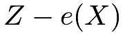
    \displaystyle E\Big[h(X)\{Z-e(X)\}\{Y-g(Z,X;\beta)\}\Big]=0 (153)

    for any function h, provided that the moment exists.

Remark: Equation (153) is the basis for parameter estimation. Consider a special case of Definition 29.4 with g(z,X;\beta)=\beta z. Choose h(X)=1 to obtain

E\{(Z-e(X))(Y-\beta Z)\}=0.

Solve for \beta to obtain

\beta=\frac{E\{(Z-e(X))Y\}}{E\{(Z-e(X))Z\}}.

Therefore, \beta equals the coefficient of Z in the TSLS of Y on Z with Z-e(X) being the IV for Z. With some basic calculations, we can also show that

\beta=\frac{\textup{cov}\{Z-e(X),Y\}}{\textup{cov}\{Z-e(X)\}}.

Therefore, \beta equals the coefficient of Z-e(X) in the OLS of Y on Z-e(X), which appeared in Chapter 72 before.

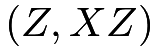
Consider another special case of Definition 29.4 with g(z,X;\beta)=(\beta_{0}+\beta_{1}^{\mkern-1.5mu\mathsf{T}}X)z. Choose h(X)=(1,X) to obtain

E\left\{\begin{pmatrix}Z-e(X)\\
(Z-e(X))X\end{pmatrix}(Y-\beta_{0}Z-\beta_{1}^{\mkern-1.5mu\mathsf{T}}XZ)\right\}=0.

That is, (\beta_{0},\beta_{1}) equal the coefficients in the TSLS of Y on (Z,XZ) with (Z-e(X),(Z-e(X))X) being the IV for (Z,XZ).

29.6 Estimation under Example 29.4

We can estimate the \beta’s by solving the empirical version of the estimating equations in Example 29.4. We first estimate the two propensity scores and obtain the centered treatment

\check{Z}_{1i}=Z_{1i}-\hat{e}(1,X_{0i})

at time point 1 and

\check{Z}_{2i}=Z_{2i}-\hat{e}(1,Z_{1i},X_{1i},X_{0i})

at time point 2.

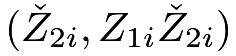
Show that we can estimate \beta_{2} and \beta_{3} by running TSLS of Y_{i} on (Z_{2i},Z_{1i}Z_{2i}) with (\check{Z}_{2i},Z_{1i}\check{Z}_{2i}) as the IV for (Z_{2i},Z_{1i}Z_{2i}), and then we can estimate \beta_{1} by running TSLS of Y_{i}-(\hat{\beta}_{2}+\hat{\beta}_{3}Z_{1i})Z_{2i} on Z_{1i} with \check{Z}_{1i} as the IV for Z_{1i}.

29.7 g-formula with a treatment at multiple time points

Extend the discussion to the setting with K time points. The temporal ordering (but not the causal diagram) of the variables is

X_{0}\rightarrow Z_{1}\rightarrow X_{1}\rightarrow Z_{2}\rightarrow\cdots\rightarrow X_{K-1}\rightarrow Z_{K}.

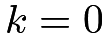
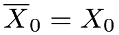
Introduce the notation \overline{Z}_{k}=(Z_{1},\ldots,Z_{k}) and \overline{X}_{k}=(X_{0},X_{1},\ldots,X_{k}) with lower case \overline{z}_{k} and \overline{x}_{k} denoting the corresponding realized values. With k=0, we have \overline{X}_{0}=X_{0} and \overline{Z}_{0} is empty. Each unit has 2^{K} potential outcomes:

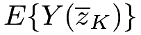
Y(\overline{z}_{K})\text{ for all }z_{1},\ldots,z_{K}=0,1.

Assume sequential ignorability below.

Assumption 29.2 (sequential ignorability at multiple time points)

We have

Z_{k}\ind Y(\overline{z}_{K})\mid(\overline{Z}_{k-1},\overline{X}_{k-1})

for all k=1,\ldots,K and all z_{1},\ldots,z_{K}=0,1.

Prove Theorem 29.6 below.

Theorem 29.6 (g-formula with multiple time points)

Under Assumption 29.2,

E\{Y(\overline{z}_{K})\}=E\left[\cdots E\{E(Y\mid\overline{z}_{K},\overline{X}_{K-1})\mid\overline{z}_{K-1},\overline{X}_{K-2}\}\cdots\mid z_{1},X_{0}\right].

Remark: In Theorem 29.6, I use the simplified notation “\overline{z}_{k}” for “\overline{Z}_{k}=\overline{z}_{k}.” With discrete X, Theorem 29.6 reduces to

\displaystyle E\{Y(\overline{z}_{K})\} \displaystyle= \displaystyle\sum_{x_{0}}\sum_{x_{1}}\cdots\sum_{x_{K-1}}E(Y\mid\overline{z}_{K},\overline{x}_{K-1})
\displaystyle\qquad\qquad\cdot\textup{pr}(x_{K-1}\mid\overline{z}_{K-1},\overline{x}_{K-2})\cdots\textup{pr}(x_{1}\mid z_{1},x_{0})\textup{pr}(x_{0});

with continuous X, Theorem 29.6 reduces to

\displaystyle E\{Y(\overline{z}_{K})\} \displaystyle= \displaystyle\int E(Y\mid\overline{z}_{K},\overline{x}_{K-1})
\displaystyle\cdot f(x_{K-1}\mid\overline{z}_{K-1},\overline{x}_{K-2})\cdots f(x_{1}\mid z_{1},x_{0})f(x_{0})\textnormal{d}\overline{x}_{K-1}.
29.8 IPW with treatments at multiple time points

Inherit the setting of Problem 29.7. Define the propensity score at K time points as

\displaystyle e(z_{1},X_{0}) \displaystyle= \displaystyle\textup{pr}(Z_{1}=z_{1}\mid X_{0}),
\displaystyle e(z_{k},\overline{Z}_{k-1},\overline{X}_{k-1}) \displaystyle= \displaystyle\textup{pr}(Z_{k}=z_{k}\mid\overline{Z}_{k-1},\overline{X}_{k-1}),
\displaystyle e(z_{K},\overline{Z}_{K-1},\overline{X}_{K-1}) \displaystyle= \displaystyle\textup{pr}(Z_{K}=z_{K}\mid\overline{Z}_{K-1},\overline{X}_{K-1}).

Prove Theorem 29.8 below assuming overlap implicitly.

Theorem 29.7 (IPW with multiple time points)

Under Assumption 29.2,

E\{Y(\overline{z}_{K})\}=E\left\{\frac{1(Z_{1}=z_{1})\cdots 1(Z_{K}=z_{K})Y}{e(z_{1},X_{0})\cdots e(z_{K},\overline{Z}_{K-1},\overline{X}_{K-1})}\right\}.

Based on Theorem 29.8, construct the Horvitz–Thompson and Hajek estimators.

29.9 MSM with treatments at multiple time points

The number of potential outcomes grows exponentially with K. The formulas in Problems 29.7 and 29.8 are not directly applicable in finite samples. We can impose the following structural assumptions on the potential outcomes.

Definition 29.5 (MSM with multiple time points)

Assume

E\{Y(\overline{z}_{K})\mid X_{0}\}=f(\overline{z}_{K},X_{0};\beta).

Two leading examples of Definition 29.5 are

E\{Y(\overline{z}_{K})\mid X_{0}\}=\beta_{0}+\beta_{1}\sum_{k=1}^{K}z_{k}+\beta_{2}^{\mkern-1.5mu\mathsf{T}}X_{0}

and

E\{Y(\overline{z}_{K})\mid X_{0}\}=\beta_{0}+\sum_{k=1}^{K}\beta_{k}z_{k}+\beta_{K+1}^{\mkern-1.5mu\mathsf{T}}X_{0}.

If we know all the potential outcomes, we can solve \beta from the following minimization problem:

\beta=\arg\min_{b}\sum_{\overline{z}_{K}}E\{Y(\overline{z}_{K})-f(\overline{z}_{K},X_{0};\beta)\}^{2}.

Theorem 29.8 below shows that under Assumption 29.2, we can solve \beta from a minimization problem that only involves observables.

Theorem 29.8 (IPW for MSM with multiple time points)

Under Assumption 29.2,

\beta=\arg\min_{b}\sum_{\overline{z}_{K}}E\left[\frac{1(Z_{1}=z_{1})\cdots 1(Z_{K}=z_{K})}{e(z_{1},X_{0})\cdots e(z_{K},\overline{Z}_{K-1},\overline{X}_{K-1})}\{Y-f(\overline{z}_{K},X_{0};\beta)\}^{2}\right].
29.10 Structural nested model with treatments at multiple time points

Inherit the setting from Problem 29.7 and the notation from Problem 29.8. This problem presents a general structural nested model.

Definition 29.6 (structural nested model with multiple time points)

The conditional effect at time k is

E\{Y(\overline{z}_{k},0)-Y(\overline{z}_{k-1},0)\mid\overline{z}_{k},\overline{X}_{k-1}\}=g_{k}(\overline{z}_{k},\overline{X}_{k-1};\beta)

for all \overline{z}_{k} and all k=1,\ldots,K.

In Definition 29.6, a logical restriction is

g_{k}(0,\overline{z}_{k-1},\overline{X}_{k-1};\beta)=0

for all \overline{z}_{k-1} and all k=1,\ldots,K.

Define

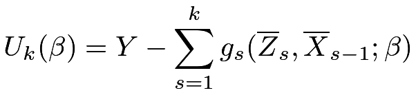
U_{k}(\beta)=Y-\sum_{s=1}^{k}g_{s}(\overline{Z}_{s},\overline{X}_{s-1};\beta)

for all k=1,\ldots,K. Theorem 29.9 below extends Theorem 29.4.

Theorem 29.9

Under Assumption 29.2 and Definition 29.6, we have

E\left[h_{k}(\overline{Z}_{k-1},\overline{X}_{k-1})\{Z_{k}-e(1,\overline{Z}_{k-1},\overline{X}_{k-1})\}U_{k}(\beta)\right]=0

for any functions h_{k} (k=1,\ldots,K), provided that the moment exists.

Remark: Choosing appropriate h_{k}’s, we can estimate \beta by solving the empirical version of Theorem 29.9.

29.11 Recommended reading

Robins et al., (2000) reviewed the MSM. Naimi et al., (2017) reviewed the g-methods.

本书:A First Course in Causal Inference,作者 Peng Ding。原文:arXiv:2305.18793v2,按 CC BY 4.0 许可发布。本站(yuanens.com)把 arXiv 网页版改成分章的纯 HTML,把公式渲染成图片,方便在 Kindle 等电子书阅读器上看,内容没有改动。转换难免有错,以原文为准。本站与作者和出版社无关。