Chapter 31 Linear and Logistic Regressions

Appendix 31.A Population ordinary least squares

Assume that (x_{i},y_{i})_{i=1}^{n}\stackrel{{\scriptstyle\textup{IID}}}{{\sim}}(x,y), where x is a p-dimensional random scalar or vector and y is a random scalar. Below I will use (x,y) to denote a general observation, dropping the subscript i for simplicity. Define the population ordinary least squares (OLS) coefficient as

\beta=\arg\min_{b}E\left\{(y-x^{\mkern-1.5mu\mathsf{T}}b)^{2}\right\}.

The objective function is quadratic in b, so we can show that the minimizer is

\beta=\left\{E\left(xx^{\mkern-1.5mu\mathsf{T}}\right)\right\}^{-1}E\left(xy\right)

if the moments exist and E(xx^{\mkern-1.5mu\mathsf{T}}) is invertible.

With \beta, we can define x^{\mkern-1.5mu\mathsf{T}}\beta as the linear projection of y on x, and define

\varepsilon=y-x^{\mkern-1.5mu\mathsf{T}}\beta (158)

as the population residual. By the definition of \beta, we can verify that

E(x\varepsilon)=E\left\{x(y-x^{\mkern-1.5mu\mathsf{T}}\beta)\right\}=E(xy)-E(xx^{\mkern-1.5mu\mathsf{T}})\beta=0.
Example 31.1 (population OLS with the intercept)

If we include 1 as a component of x, then

E(\varepsilon)=E(y-x^{\mkern-1.5mu\mathsf{T}}\beta)=0

which further implies that \textup{cov}(x,\varepsilon)=0. So with an intercept in \beta, the mean of the population residual must be zero, and it is uncorrelated with other covariates by construction.

Example 31.2 (univariate population OLS with the intercept)

An important special case is that for scalars x and y, we can define

(\alpha,\beta)=\arg\min_{a,b}E\{(y-a-bx)^{2}\}

which have explicit formulas

\beta=\frac{\textup{cov}(x,y)}{\textup{var}(x)},\quad\alpha=E(y)-\beta E(x).
Example 31.3 (univariate population OLS without an intercept)

Without intercept, we can define

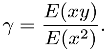
\gamma=\arg\min_{c}E\{(y-cx)^{2}\}

which equals

\gamma=\frac{E(xy)}{E(x^{2})}.

When x has mean zero, \gamma equals the \beta in Example 31.2.

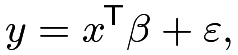
We can also rewrite (158) as

y=x^{\mkern-1.5mu\mathsf{T}}\beta+\varepsilon, (159)

which holds by the definition of the population OLS coefficient and residual without any modeling assumption. We call (159) the population OLS decomposition.

Appendix 31.B Sample ordinary least squares

Based on data (x_{i},y_{i})_{i=1}^{n}\stackrel{{\scriptstyle\textup{IID}}}{{\sim}}(x,y), we can easily obtain the moment estimator for the population OLS coefficient

\hat{\beta}=\left(n^{-1}\sum_{i=1}^{n}x_{i}x_{i}^{\mkern-1.5mu\mathsf{T}}\right)^{-1}\left(n^{-1}\sum_{i=1}^{n}x_{i}y_{i}\right),

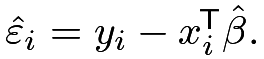
and the residuals \hat{\varepsilon}_{i}=y_{i}-x_{i}^{\mkern-1.5mu\mathsf{T}}\hat{\beta}. This is called the sample OLS or simply the OLS. The OLS coefficient \hat{\beta} minimizes the residual sum of squares
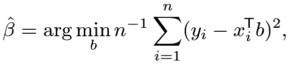
\hat{\beta}=\arg\min_{b}n^{-1}\sum_{i=1}^{n}(y_{i}-x_{i}^{\mkern-1.5mu\mathsf{T}}b)^{2},

so it must satisfy

\sum_{i=1}^{n}x_{i}(y_{i}-x_{i}^{\mkern-1.5mu\mathsf{T}}\hat{\beta})=0,

which is sometimes called the Normal equation. The fitted values, also called the linear projections of y_{i} on x_{i}, equal

\hat{y}_{i}=x_{i}^{\mkern-1.5mu\mathsf{T}}\hat{\beta}\quad(i=1,\ldots,n).

Using the matrix notation

X=\begin{pmatrix}x_{1}^{\mkern-1.5mu\mathsf{T}}\\
\vdots\\
x_{n}^{\mkern-1.5mu\mathsf{T}}\end{pmatrix},\quad Y=\begin{pmatrix}y_{1}\\
\vdots\\
y_{n}\end{pmatrix},

we can write the OLS coefficient as

\hat{\beta}=(X^{\mkern-1.5mu\mathsf{T}}X)^{-1}X^{\mkern-1.5mu\mathsf{T}}Y

and the fitted vector as

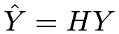
\hat{Y}=X\hat{\beta}=X(X^{\mkern-1.5mu\mathsf{T}}X)^{-1}X^{\mkern-1.5mu\mathsf{T}}Y.

Define the hat matrix as

H=X(X^{\mkern-1.5mu\mathsf{T}}X)^{-1}X^{\mkern-1.5mu\mathsf{T}}.

Then we also have \hat{Y}=HY, justifying the name “hat matrix.” The diagonal elements of H, h_{ii}’s, are often called the leverage scores.

Assuming finite fourth moments of (x,y), we can use the law of large numbers and the CLT to show that

\sqrt{n}(\hat{\beta}-\beta)\rightarrow\text{N}(0,V)

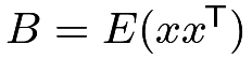
in distribution with V=B^{-1}MB^{-1}, where B=E(xx^{\mkern-1.5mu\mathsf{T}}) and M=E(\varepsilon^{2}xx^{\mkern-1.5mu\mathsf{T}}). So a moment estimator for the asymptotic variance of \hat{\beta} is

\hat{V}_{\textsc{ehw}}=n^{-1}\left(n^{-1}\sum_{i=1}^{n}x_{i}x_{i}^{\mkern-1.5mu\mathsf{T}}\right)^{-1}\left(n^{-1}\sum_{i=1}^{n}\hat{\varepsilon}_{i}^{2}x_{i}x_{i}^{\mkern-1.5mu\mathsf{T}}\right)\left(n^{-1}\sum_{i=1}^{n}x_{i}x_{i}^{\mkern-1.5mu\mathsf{T}}\right)^{-1}, (160)

which is called the Eicker–Huber–White (EHW) robust covariance estimator (Eicker,, 1967; Huber,, 1967; White,, 1980). We can show that n\hat{V}_{\textsc{ehw}}\rightarrow V in probability. Based on \hat{\beta} and \hat{V}_{\textsc{ehw}}, we can make inference about the population OLS coefficient \beta.

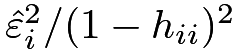
There are many variants of the EHW robust covariance estimator based on the leverage scores (Long and Ervin,, 2000). In particular, the HC1 variant modifies \hat{\varepsilon}_{i}^{2} to \hat{\varepsilon}_{i}^{2}/(n-p), the HC2 variant modifies \hat{\varepsilon}_{i}^{2} to \hat{\varepsilon}_{i}^{2}/(1-h_{ii}), and the HC3 variant modifies \hat{\varepsilon}_{i}^{2} to \hat{\varepsilon}_{i}^{2}/(1-h_{ii})^{2}, in the definition of \hat{V}_{\textsc{ehw}}.

Appendix 31.C Frisch–Waugh–Lovell Theorem

The Frisch–Waugh–Lovell (FWL) theorem has two versions: one at the population level and the other at the sample level. It reduces multivariate OLS to univariate OLS and therefore facilitates the understanding and calculation of the OLS coefficients. Below I will present special cases of the FWL theorem which are enough for this book.

Theorem 31.1 (population FWL)

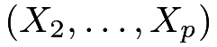
The coefficient of x_{1} in the OLS fit of y on (x_{1},x_{2},\ldots,x_{p}) equals the coefficient of \tilde{x}_{1} in the OLS fit of y or \tilde{y} on \tilde{x}_{1}, where \tilde{y} is the residual from the OLS fit of y on (x_{2},\ldots,x_{p}) and \tilde{x}_{1} is the residual from the OLS fit of x_{1} on (x_{2},\ldots,x_{p}).

In Theorem 31.1, residualizing x_{1} is crucial but residualizing y is not.

Theorem 31.2 (sample FWL)

With data (Y,X_{1},X_{2},\ldots,X_{p}) containing column vectors, the coefficient of X_{1} in the OLS fit of Y on (X_{1},X_{2},\ldots,X_{p}) equals the coefficient of \tilde{X}_{1} in the OLS fit of Y or \tilde{Y} on \tilde{X}_{1}, where \tilde{Y} is the residual vector from the OLS fit of Y on (X_{2},\ldots,X_{p}) and \tilde{X}_{1} is the residual vector from the OLS fit of X_{1} on (X_{2},\ldots,X_{p}).

Again, in Theorem 31.2, residualizing X_{1} is crucial but residualizing Y is not. Ding, (2021) gives more numerical properties related to the sample FWL theorem.

Appendix 31.D Linear model

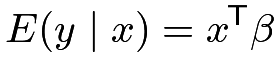
Sometimes, we impose a stronger model assumption which requires the conditional mean of y given x is linear:

E(y\mid x)=x^{\mkern-1.5mu\mathsf{T}}\beta

or, equivalently,

y=x^{\mkern-1.5mu\mathsf{T}}\beta+\varepsilon\qquad\text{with}\qquad E(\varepsilon\mid x)=0,

which is called the restricted mean model. Under this model, the population OLS coefficient is the true parameter of interest:

\displaystyle\left\{E(xx^{\mkern-1.5mu\mathsf{T}})\right\}^{-1}E(xy) \displaystyle=\left\{E(xx^{\mkern-1.5mu\mathsf{T}})\right\}^{-1}E\left\{xE(y\mid x)\right\}
\displaystyle=\left\{E(xx^{\mkern-1.5mu\mathsf{T}})\right\}^{-1}E(xx^{\mkern-1.5mu\mathsf{T}}\beta)
\displaystyle=\beta.

Moreover, the population OLS coefficient does not depend on the distribution of x. The asymptotic inference in Section 31.A applies to this model too.

In the special case with \textup{var}(\varepsilon\mid x)=\sigma^{2}, the asymptotic variance of the OLS coefficient reduces to

V=\sigma^{2}\{E(xx^{\mkern-1.5mu\mathsf{T}})\}^{-1}

so a simpler moment estimator for the asymptotic variance of \hat{\beta} is

\hat{V}_{\textsc{ols}}=\hat{\sigma}^{2}\left(\sum_{i=1}^{n}x_{i}x_{i}^{\mkern-1.5mu\mathsf{T}}\right)^{-1} (161)

where \hat{\sigma}^{2}=(n-p)^{-1}\sum_{i=1}^{n}\hat{\varepsilon}_{i}^{2} is an unbiased estimator for \sigma^{2}, recalling that n denotes the sample size and p denotes the dimension of x. This is the standard covariance estimator from the lm function.

Based on the BostonHousing data, we first obtain the standard output from the lm function.

> library("mlbench")
> data(BostonHousing)
> ols.fit = lm(medv ~ ., data = BostonHousing)
> summary(ols.fit)
Call:
lm(formula = medv ~ ., data = BostonHousing)
Residuals:
Min 1Q Median 3Q Max
-15.595 -2.730 -0.518 1.777 26.199
Coefficients:
Estimate Std. Error t value Pr(>|t|)
(Intercept) 3.646e+01 5.103e+00 7.144 3.28e-12 ***
crim -1.080e-01 3.286e-02 -3.287 0.001087 **
zn 4.642e-02 1.373e-02 3.382 0.000778 ***
indus 2.056e-02 6.150e-02 0.334 0.738288
chas1 2.687e+00 8.616e-01 3.118 0.001925 **
nox -1.777e+01 3.820e+00 -4.651 4.25e-06 ***
rm 3.810e+00 4.179e-01 9.116 < 2e-16 ***
age 6.922e-04 1.321e-02 0.052 0.958229
dis -1.476e+00 1.995e-01 -7.398 6.01e-13 ***
rad 3.060e-01 6.635e-02 4.613 5.07e-06 ***
tax -1.233e-02 3.760e-03 -3.280 0.001112 **
ptratio -9.527e-01 1.308e-01 -7.283 1.31e-12 ***
b 9.312e-03 2.686e-03 3.467 0.000573 ***
lstat -5.248e-01 5.072e-02 -10.347 < 2e-16 ***

In R, the lm function can compute \hat{\beta}, and the hccm function in the package car can compute \hat{V}_{\textsc{ehw}} as well as its variants. Below we compare the t-statistics based on different choices of the standard errors. In this example, the EHW standard errors differ a lot for some regression coefficients.

> library("car")
> ols.fit.hc0 = sqrt(diag(hccm(ols.fit, type = "hc0")))
> ols.fit.hc1 = sqrt(diag(hccm(ols.fit, type = "hc1")))
> ols.fit.hc2 = sqrt(diag(hccm(ols.fit, type = "hc2")))
> ols.fit.hc3 = sqrt(diag(hccm(ols.fit, type = "hc3")))
> tvalues = summary(ols.fit)$coef[,1]/
+ cbind(summary(ols.fit)$coef[,2],
+ ols.fit.hc0,
+ ols.fit.hc1,
+ ols.fit.hc2,
+ ols.fit.hc3)
> colnames(tvalues) = c("ols", "hc0", "hc1", "hc2", "hc3")
> round(tvalues, 2)
ols hc0 hc1 hc2 hc3
(Intercept) 7.14 4.62 4.56 4.48 4.33
crim -3.29 -3.78 -3.73 -3.48 -3.17
zn 3.38 3.42 3.37 3.35 3.27
indus 0.33 0.41 0.41 0.41 0.40
chas1 3.12 2.11 2.08 2.05 2.00
nox -4.65 -4.76 -4.69 -4.64 -4.53
rm 9.12 4.57 4.51 4.43 4.28
age 0.05 0.04 0.04 0.04 0.04
dis -7.40 -6.97 -6.87 -6.81 -6.66
rad 4.61 5.05 4.98 4.91 4.76
tax -3.28 -4.65 -4.58 -4.54 -4.43
ptratio -7.28 -8.23 -8.11 -8.06 -7.89
b 3.47 3.53 3.48 3.44 3.34
lstat -10.35 -5.34 -5.27 -5.18 -5.01

Appendix 31.E Weighted least squares

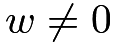
Assuming that (w_{i},x_{i},y_{i})\stackrel{{\scriptstyle\textup{IID}}}{{\sim}}(w,x,y) with w\neq 0. At the population level, we can define the weighted least squares (WLS) coefficient as

\beta_{w}=\arg\min_{b}E\{w(y-x^{\mkern-1.5mu\mathsf{T}}b)^{2}\},

which satisfies

E\{wx(y-x^{\mkern-1.5mu\mathsf{T}}\beta_{w})\}=0

and thus equals

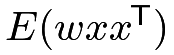
\beta_{w}=\{E(wxx^{\mkern-1.5mu\mathsf{T}})\}^{-1}E(wxy)

if E(wxx^{\mkern-1.5mu\mathsf{T}}) is invertible.

At the sample level, we can define the WLS coefficient as

\hat{\beta}_{w}=\arg\min_{b}\sum_{i=1}^{n}w_{i}(y_{i}-x_{i}^{\mkern-1.5mu\mathsf{T}}b)^{2},

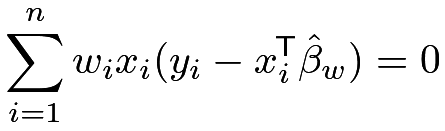
which satisfies

\sum_{i=1}^{n}w_{i}x_{i}(y_{i}-x_{i}^{\mkern-1.5mu\mathsf{T}}\hat{\beta}_{w})=0

and thus equals

\hat{\beta}_{w}=\left(n^{-1}\sum_{i=1}^{n}w_{i}x_{i}x_{i}^{\mkern-1.5mu\mathsf{T}}\right)^{-1}\left(n^{-1}\sum_{i=1}^{n}w_{i}x_{i}y_{i}\right)

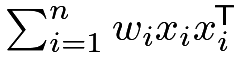
if \sum_{i=1}^{n}w_{i}x_{i}x_{i}^{\mkern-1.5mu\mathsf{T}} is invertible.

In R, we can specify weights in the lm function to implement WLS.

Appendix 31.F Logistic regression

31.F.1 Model

Technically, we can apply the OLS procedure even if the outcome y is binary. However, it is a little awkward to have predicted probabilities outside the range of [0,1]. This motivates us to consider the following model:

\textup{pr}(y_{i}=1\mid x_{i})=g(x_{i}^{\mkern-1.5mu\mathsf{T}}\beta),

where g(\cdot):\mathbb{R}\rightarrow[0,1] is a monotone function, and its inverse is often called the link function. The g(\cdot) function can be any distribution function of a random variable, but we will focus on the logistic form:

g(z)=\frac{e^{z}}{1+e^{z}}=(1+e^{-z})^{-1}.

We can also write the logistic model as
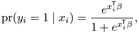
\textup{pr}(y_{i}=1\mid x_{i})=\frac{e^{x_{i}^{\mkern-1.5mu\mathsf{T}}\beta}}{1+e^{x_{i}^{\mkern-1.5mu\mathsf{T}}\beta}},

or, equivalently, with the definition \text{logit}(z)=\log\frac{z}{1-z}, we have

\text{logit}\left\{\textup{pr}(y_{i}=1\mid x_{i})\right\}=x_{i}^{\mkern-1.5mu\mathsf{T}}\beta.

Assume that x_{i1} is binary. Under the logistic model, we have

\displaystyle\beta_{1} \displaystyle= \displaystyle\text{logit}\left\{\textup{pr}(y_{i}=1\mid x_{i1}=1,\ldots)\right\}-\text{logit}\left\{\textup{pr}(y_{i}=1\mid x_{i1}=0,\ldots)\right\}
\displaystyle= \displaystyle\log\frac{\textup{pr}(y_{i}=1\mid x_{i1}=1,\ldots)/\textup{pr}(y_{i}=0\mid x_{i1}=1,\ldots)}{\textup{pr}(y_{i}=1\mid x_{i1}=0,\ldots)/\textup{pr}(y_{i}=0\mid x_{i1}=0,\ldots)},

where \ldots contains all other regressor x_{i2},\ldots,x_{ip}. Therefore, the coefficient \beta_{1} equals the log of the odds ratio of x_{i1} on y_{i} conditional on other regressors.

31.F.2 Maximum likelihood estimate

Let \textup{pr}(y_{i}=1\mid x_{i})=\pi(x_{i},\beta). To estimate the parameter \beta, we can maximize the following likelihood function:

\displaystyle L(\beta) \displaystyle=\prod_{i=1}^{n}\left\{\pi(x_{i},\beta)\right\}^{y_{i}}\left\{1-\pi(x_{i},\beta)\right\}^{1-y_{i}}
\displaystyle=\prod_{i=1}^{n}\left\{\frac{\pi(x_{i},\beta)}{1-\pi(x_{i},\beta)}\right\}^{y_{i}}\left\{1-\pi(x_{i},\beta)\right\}
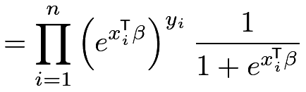
\displaystyle=\prod_{i=1}^{n}\left(e^{x_{i}^{\mkern-1.5mu\mathsf{T}}\beta}\right)^{y_{i}}\frac{1}{1+e^{x_{i}^{\mkern-1.5mu\mathsf{T}}\beta}}
\displaystyle=\prod_{i=1}^{n}\frac{e^{y_{i}x_{i}^{\mkern-1.5mu\mathsf{T}}\beta}}{1+e^{x_{i}^{\mkern-1.5mu\mathsf{T}}\beta}}.

Let \hat{\beta} denote the maximizer, which is called the maximum likelihood estimate (MLE). Taking the log of L(\beta) and differentiating it with respect to \beta, we can show that the MLE must satisfy the first-order condition:
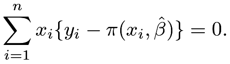
\sum_{i=1}^{n}x_{i}\{y_{i}-\pi(x_{i},\hat{\beta})\}=0.

If x_{i} contains the intercept, the MLE must satisfy
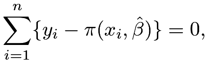
\sum_{i=1}^{n}\{y_{i}-\pi(x_{i},\hat{\beta})\}=0,

that is, the average of the observed y_{i}’s must be identical to the average of the fitted probabilities \pi(x_{i},\hat{\beta})’s.

Using the general theory for the MLE, we can show that it is consistent for the true parameter \beta and is asymptotically Normal:

\sqrt{n}(\hat{\beta}-\beta)\rightarrow\text{N}(0,V)

in distribution, where V=E[\pi(x_{i},\beta)\{1-\pi(x_{i},\beta)\}xx^{\mkern-1.5mu\mathsf{T}}]. So we can approximate the covariance matrix of \hat{\beta} by

n^{-1}\sum_{i=1}^{n}\pi(x_{i},\hat{\beta})\{1-\pi(x_{i},\hat{\beta})\}x_{i}x_{i}^{\mkern-1.5mu\mathsf{T}}.

In R, the glm function can find the MLE and report the estimated covariance matrix. We use the lalonde data to illustrate the logistic regression with the binary outcome indicating positive real earnings in 1978.

> library(Matching)
> data(lalonde)
> logit.re78 = glm(I(re78>0) ~ ., family = binomial,
+ data = lalonde)
> summary(logit.re78)
Call:
glm(formula = I(re78 > 0) ~ ., family = binomial, data = lalonde)
Deviance Residuals:
Min 1Q Median 3Q Max
-2.1789 -1.3170 0.7568 0.9413 1.0882
Coefficients:
Estimate Std. Error z value Pr(>|z|)
(Intercept) 1.910e+00 1.241e+00 1.539 0.1238
age -2.812e-03 1.533e-02 -0.183 0.8545
educ -2.179e-02 7.831e-02 -0.278 0.7808
black -1.060e+00 5.041e-01 -2.103 0.0354 *
hisp 2.741e-01 6.967e-01 0.393 0.6940
married 7.577e-02 3.057e-01 0.248 0.8042
nodegr -1.984e-01 3.460e-01 -0.573 0.5664
re74 7.857e-06 3.173e-05 0.248 0.8044
re75 4.016e-05 6.058e-05 0.663 0.5074
u74 -6.177e-02 4.095e-01 -0.151 0.8801
u75 1.505e-02 3.518e-01 0.043 0.9659
treat 5.412e-01 2.222e-01 2.435 0.0149 *
31.F.3 Extension to the case-control study

In case-control studies, sampling is conditional on the binary outcome, that is, units with outcomes y_{i}=1 and y_{i}=0 are sampled with different probabilities. Let s_{i} be the sampling indicator. In case-control studies, we have

\textup{pr}(s_{i}=1\mid x_{i},y_{i})=\textup{pr}(s_{i}=1\mid y_{i})

as a function of y_{i}, and we only observe units with s_{i}=1.

Based on the model and the sampling mechanism of the case-control study, it does not seem obvious whether or not we can still use logistic regression to estimate the coefficients. Nevertheless, Prentice and Pyke, (1979) proved a positive results. In case-control studies, logistic regression can still consistently estimate all the coefficients except for the intercept.

31.F.4 Logistic regression with weights

Sometimes, unit i has weight w_{i}. Then we can fit a weighted logistic regression by solving
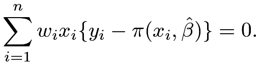
\sum_{i=1}^{n}w_{i}x_{i}\{y_{i}-\pi(x_{i},\hat{\beta})\}=0.

In R, we can specify weights in the glm function to implement weighted logistic regression.

Appendix 31.G Homework problems

AE.1 Sample WLS with the intercept

Assume the regressor x_{i} contains the intercept. Show that

\bar{y}_{w}=\bar{x}_{w}^{\mkern-1.5mu\mathsf{T}}\hat{\beta}_{w} (162)

where \bar{x}_{w}=\sum_{i=1}^{n}w_{i}x_{i}/\sum_{i=1}^{n}w_{i} and \bar{y}_{w}=\sum_{i=1}^{n}w_{i}y_{i}/\sum_{i=1}^{n}w_{i} are the weighted averages of the x_{i}’s and y_{i}’s.

AE.2 Population OLS with a binary regressor

Assume x is binary. Define the population OLS:

(\alpha,\beta)=\arg\min_{(a,b)}E\{(y-a-bx)^{2}\}.

Show that \beta=E(y\mid x=1)-E(y\mid x=0) and \alpha=E(y\mid x=0).

AE.3 Univariate WLS

As a special case of WLS, define

(\hat{\alpha}_{w},\hat{\beta}_{w})=\arg\min_{(a,b)}\sum_{i=1}^{n}w_{i}(y_{i}-a-bx_{i})^{2}

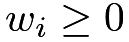
where w_{i}\geq 0. Show that

\displaystyle\hat{\beta}_{w}=\frac{\sum_{i=1}^{n}w_{i}(x_{i}-\bar{x}_{w})(y_{i}-\bar{y}_{w})}{\sum_{i=1}^{n}w_{i}(x_{i}-\bar{x}_{w})^{2}} (163)

and

\displaystyle\hat{\alpha}_{w}=\bar{y}_{w}-\hat{\beta}_{w}\bar{x}_{w}, (164)

where \bar{x}_{w}=\sum_{i=1}^{n}w_{i}x_{i}/\sum_{i=1}^{n}w_{i} and \bar{y}_{w}=\sum_{i=1}^{n}w_{i}y_{i}/\sum_{i=1}^{n}w_{i} are the weighted averages of the x_{i}’s and y_{i}’s.

Further assume that the x_{i}’s are binary. Show that

\displaystyle\hat{\beta}_{w}=\frac{\sum_{i=1}^{n}w_{i}x_{i}y_{i}}{\sum_{i=1}^{n}w_{i}x_{i}}-\frac{\sum_{i=1}^{n}w_{i}(1-x_{i})y_{i}}{\sum_{i=1}^{n}w_{i}(1-x_{i})}. (165)

That is, if the regressor is binary in the univariate WLS, the coefficient of the regressor equals the difference in the weighted means.

Remark: To prove (165), use an appropriate reparametrization of the WLS problem. Otherwise, the derivation can be tedious.

AE.4 OLS with orthogonal regressors

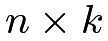
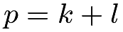
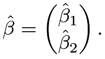
Consider sample OLS fit of an n-vector Y on an n\times p matrix X, with coefficient \hat{\beta}. Partition X into X=(X_{1},X_{2}), where X_{1} is an n\times k matrix and X_{2} is an n\times l matrix, with p=k+l. Correspondingly, partition \hat{\beta} into

\hat{\beta}=\begin{pmatrix}\hat{\beta}_{1}\\
\hat{\beta}_{2}\end{pmatrix}.

Assume X_{1} and X_{2} are orthogonal, that is, X_{1}^{\mkern-1.5mu\mathsf{T}}X_{2}=0. Show that \hat{\beta}_{1} equals the coefficient from OLS of Y on X_{1} and \hat{\beta}_{2} equals the coefficient from OLS of Y on X_{2}, respectively.

AE.5 OLS with a non-degenerate transformation of the regressors

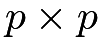
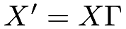
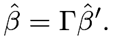
Define \hat{\beta} as the coefficient from the sample OLS fit of an n-vector Y on an n\times p matrix X. Let \Gamma be a p\times p non-degenerate matrix, and define X^{\prime}=X\Gamma. Define \hat{\beta}^{\prime} as the coefficient from the sample OLS fit of Y on X^{\prime}.

Show that

\hat{\beta}=\Gamma\hat{\beta}^{\prime}.
AE.6 Variances of the OLS estimator

Assume (x_{i},y_{i})_{i=1}^{n}\stackrel{{\scriptstyle\textup{IID}}}{{\sim}}(x,y) and

E(y\mid x)=x^{\mkern-1.5mu\mathsf{T}}\beta,\quad\textup{var}(y\mid x)=\sigma^{2}(x).

Show that the OLS estimator \hat{\beta} has conditional mean

E(\hat{\beta}\mid x_{1},\ldots,x_{n})=\beta

and conditional variance

\textup{var}(\hat{\beta}\mid x_{1},\ldots,x_{n})=\left(\sum_{i=1}^{n}x_{i}x_{i}^{\mkern-1.5mu\mathsf{T}}\right)^{-1}\left(\sum_{i=1}^{n}\sigma^{2}(x_{i})x_{i}x_{i}^{\mkern-1.5mu\mathsf{T}}\right)\left(\sum_{i=1}^{n}x_{i}x_{i}^{\mkern-1.5mu\mathsf{T}}\right)^{-1}.

Remark: This problem may provide some intuition for the variance estimators (160) and (161).

本书:A First Course in Causal Inference,作者 Peng Ding。原文:arXiv:2305.18793v2,按 CC BY 4.0 许可发布。本站(yuanens.com)把 arXiv 网页版改成分章的纯 HTML,把公式渲染成图片,方便在 Kindle 等电子书阅读器上看,内容没有改动。转换难免有错,以原文为准。本站与作者和出版社无关。