Chapter 13 The Average Causal Effect on the Treated Units and Other Estimands

Chapters 10–12 focused on the identification and estimation of the average causal effect \tau=E\{Y(1)-Y(0)\} under the ignorability and overlap assumptions. Conceptually, it is straightforward to extend the discussion to the average causal effects on the treated and control units:

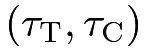
\displaystyle\tau_{\textsc{T}} \displaystyle= \displaystyle E\{Y(1)-Y(0)\mid Z=1\},
\displaystyle\tau_{\textsc{C}} \displaystyle= \displaystyle E\{Y(1)-Y(0)\mid Z=0\}.

If \tau_{\textsc{T}} and \tau_{\textsc{C}} differ from \tau, then the average causal effects are heterogeneous across the treatment and control groups. Whether we should estimate \tau_{\textsc{T}}, \tau_{\textsc{C}} or \tau depends on the practical question of interest.

Because of the symmetry, this chapter focuses on \tau_{\textsc{T}}. Chapter 70 also discusses extensions to other estimands.

67 Nonparametric identification of \tau_{\textsc{T}}

The average causal effect on the treated units equals

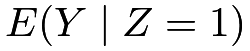
\tau_{\textsc{T}}=E(Y\mid Z=1)-E\{Y(0)\mid Z=1\},

where the first term E(Y\mid Z=1) is directly identifiable from the data and the second term E\{Y(0)\mid Z=1\} is counterfactual. The key assumption to identify the second term is the following ignorability and overlap assumptions.

Assumption 13.1
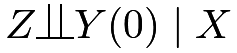
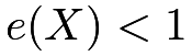
Z\ind Y(0)\mid X and e(X)<1.

Because the key is to identify E\{Y(0)\mid Z=1\}, we only need the “one-sided” ignorability and overlap assumptions. Under Assumption 13.1, we have the following identification result for \tau_{\textsc{T}}.

Theorem 13.1

Under Assumption 13.1, we have

\displaystyle E\{Y(0)\mid Z=1\} \displaystyle= \displaystyle E\left\{E(Y\mid Z=0,X)\mid Z=1\right\}
\displaystyle= \displaystyle\int E(Y\mid Z=0,X=x)f(x\mid Z=1)\textup{d}x.

By Theorem 13.1 the counterfactual mean E\{Y(0)\mid Z=1\} equals the conditional mean of the observed outcomes under the control, averaged over the distribution of the covariates under the treatment. It implies that \tau_{\textsc{T}} is nonparametrically identified by

\tau_{\textsc{T}}=E(Y\mid Z=1)-E\left\{E(Y\mid Z=0,X)\mid Z=1\right\} (70)

Proof of Theorem 13.1: We have

\displaystyle E\{Y(0)\mid Z=1\} \displaystyle= \displaystyle E\big[E\{Y(0)\mid Z=1,X\}\mid Z=1\big]
\displaystyle= \displaystyle E\big[E\{Y(0)\mid Z=0,X\}\mid Z=1\big]
\displaystyle= \displaystyle E\left\{E(Y\mid Z=0,X)\mid Z=1\right\}
\displaystyle= \displaystyle\int E(Y\mid Z=0,X=x)f(x\mid Z=1)\textup{d}x.

\square

With a discrete X, the identification formula in Theorem 13.1 reduces to

E\{Y(0)\mid Z=1\}=\sum_{k=1}^{K}E(Y\mid Z=0,X=k)\textup{pr}(X=k\mid Z=1),

motivating the following stratified estimator for \tau_{\textsc{T}}:

\hat{\tau}_{\textsc{T}}=\hat{\bar{Y}}(1)-\sum_{k=1}^{K}\hat{\pi}_{[k]\mid 1}\hat{\bar{Y}}_{[k]}(0),

where \hat{\pi}_{[k]\mid 1}=n_{[k]1}/n_{1} is the proportion of category k of X among the treated units.

For continuous X, we need to fit an outcome model for E(Y\mid Z=0,X) using the control units. If the fitted values for the control potential outcomes are \hat{\mu}_{0}(X_{i}), then the outcome regression estimator is
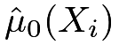

\hat{\tau}_{\textsc{T}}^{\text{reg}}=\hat{\bar{Y}}(1)-n_{1}^{-1}\sum_{i=1}^{n}Z_{i}\hat{\mu}_{0}(X_{i})=n_{1}^{-1}\sum_{i=1}^{n}Z_{i}\{Y_{i}-\hat{\mu}_{0}(X_{i})\}.
Example 13.1

If we specify a linear model for all units

E(Y\mid Z,X)=\beta_{0}+\beta_{z}Z+\beta_{x}^{\mkern-1.5mu\mathsf{T}}X,

then

\displaystyle\tau_{\textsc{T}} \displaystyle= \displaystyle E\{E(Y\mid Z=1,X)-E(Y\mid Z=0,X)\mid Z=1\}
\displaystyle= \displaystyle\beta_{z}.

If we run OLS to obtain (\hat{\beta}_{0},\hat{\beta}_{z},\hat{\beta}_{x}), then we can use \hat{\beta}_{z} to estimate \tau_{\textsc{T}}. Section 56.2 shows that \hat{\beta}_{z} is an estimator for \tau, and this example further shows that \hat{\beta}_{z} is an estimator for \tau_{\textsc{T}}. This is not surprising because the linear model assumes constant causal effects across units.

Example 13.2

The identification formula depends only on E(Y\mid Z=0,X), so we need only to specify a model for the control units. When this model is linear,

E(Y\mid Z=0,X)=\beta_{0\mid 0}+\beta_{x\mid 0}^{\mkern-1.5mu\mathsf{T}}X,

we have

\displaystyle\tau_{\textsc{T}} \displaystyle= \displaystyle E(Y\mid Z=1)-E(\beta_{0\mid 0}+\beta_{x\mid 0}^{\mkern-1.5mu\mathsf{T}}X\mid Z=1)
\displaystyle= \displaystyle E(Y\mid Z=1)-\beta_{0\mid 0}-\beta_{x\mid 0}^{\mkern-1.5mu\mathsf{T}}E(X\mid Z=1).

If we run OLS with only the control units to obtain (\hat{\beta}_{0\mid 0},\hat{\beta}_{x\mid 0}), then the estimator is

\hat{\tau}_{\textsc{T}}=\hat{\bar{Y}}(1)-\hat{\beta}_{0\mid 0}-\hat{\beta}_{x\mid 0}^{\mkern-1.5mu\mathsf{T}}\hat{\bar{X}}(1).

Using the property of the OLS (see 162), we have

\hat{\bar{Y}}(0)=\hat{\beta}_{0\mid 0}+\hat{\beta}_{x\mid 0}^{\mkern-1.5mu\mathsf{T}}\hat{\bar{X}}(0).

Therefore, the above estimator reduces to

\hat{\tau}_{\textsc{T}}=\left\{\hat{\bar{Y}}(1)-\hat{\bar{Y}}(0)\right\}-\hat{\beta}_{x\mid 0}^{\mkern-1.5mu\mathsf{T}}\left\{\hat{\bar{X}}(1)-\hat{\bar{X}}(0)\right\},

which is similar to () with a different coefficient for the difference in means of the covariates.

As an algebraic fact, we can show that this estimator equals the coefficient of Z in the OLS fit of the outcome on the treatment, covariates, and their interactions, with the covariates centered as X_{i}-\hat{\bar{X}}(1). See Problem 13.2 for more details.

68 Inverse propensity score weighting and doubly robust estimation of \tau_{\textsc{T}}

Theorem 13.2

Under Assumption 13.1, we have

\displaystyle E\{Y(0)\mid Z=1\}=E\left\{\frac{e(X)}{e}\frac{1-Z}{1-e(X)}Y\right\} (71)

and

\displaystyle\tau_{\textsc{T}}=E(Y\mid Z=1)-E\left\{\frac{e(X)}{e}\frac{1-Z}{1-e(X)}Y\right\}, (72)

where e=\textup{pr}(Z=1) is the marginal probability of the treatment.

Proof of Theorem 13.2: The left-hand side of (71) equals

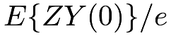
\displaystyle E\{Y(0)\mid Z=1\} \displaystyle= \displaystyle E\{ZY(0)\}/e
\displaystyle= \displaystyle E\big[E(Z\mid X)E\{Y(0)\mid X\}\big]/e
\displaystyle= \displaystyle E\big[e(X)E\{Y(0)\mid X\}\big]/e.

The right-hand side of (71) equals

\displaystyle E\left\{\frac{e(X)}{e}\frac{1-Z}{1-e(X)}Y\right\} \displaystyle= \displaystyle E\left[E\left\{\frac{e(X)}{e}\frac{1-Z}{1-e(X)}Y(0)\mid X\right\}\right]
\displaystyle= \displaystyle E\left[\frac{e(X)}{e\{1-e(X)\}}E\left\{(1-Z)Y(0)\mid X\right\}\right]
\displaystyle= \displaystyle E\left[\frac{e(X)}{e\{1-e(X)\}}E(1-Z\mid X)E\left\{Y(0)\mid X\right\}\right]
\displaystyle= \displaystyle E\big[e(X)E\{Y(0)\mid X\}\big]/e.

So (71) holds. \square

We have two IPW estimators

\hat{\tau}_{\textsc{T}}^{\text{ht}}=\hat{\bar{Y}}(1)-n_{1}^{-1}\sum_{i=1}^{n}\hat{o}(X_{i})(1-Z_{i})Y_{i}

and

\hat{\tau}_{\textsc{T}}^{\text{hajek}}=\hat{\bar{Y}}(1)-\frac{\sum_{i=1}^{n}\hat{o}(X_{i})(1-Z_{i})Y_{i}}{\sum_{i=1}^{n}\hat{o}(X_{i})(1-Z_{i})},

where \hat{o}(X_{i})=\hat{e}(X_{i})/\{1-\hat{e}(X_{i})\} is the fitted odds of the treatment given covariates.

We also have a doubly robust estimator for E\{Y(0)\mid Z=1\} which combines the propensity score and the outcome models. Define

\displaystyle\tilde{\mu}_{0\textsc{T}}^{\textup{dr}}=E\left[o(X,\alpha)(1-Z)\{Y-\mu_{0}(X,\beta_{0})\}+Z\mu_{0}(X,\beta_{0})\right]/e, (73)

where o(X,\alpha)=e(X,\alpha)/\{1-e(X,\alpha)\}.

Theorem 13.3

Under Assumption 13.1, if either e(X,\alpha)=e(X) or \mu_{0}(X,\beta_{0})=\mu_{0}(X), then \mu_{0\textsc{T}}^{\text{dr}}=E\{Y(0)\mid Z=1\}.

Proof of Theorem 13.3: We have the decomposition

\displaystyle e\left[\tilde{\mu}_{0\textsc{T}}^{\text{dr}}-E\{Y(0)\mid Z=1\}\right]
\displaystyle= \displaystyle E\left[o(X,\alpha)(1-Z)\{Y(0)-\mu_{0}(X,\beta_{0})\}+Z\mu_{0}(X,\beta_{0})\right]-E\{ZY(0)\}
\displaystyle= \displaystyle E\left[o(X,\alpha)(1-Z)\{Y(0)-\mu_{0}(X,\beta_{0})\}-Z\{Y(0)-\mu_{0}(X,\beta_{0})\}\right]
\displaystyle= \displaystyle E\left[\left\{o(X,\alpha)(1-Z)-Z\right\}\{Y(0)-\mu_{0}(X,\beta_{0})\}\right]
\displaystyle= \displaystyle E\left[\frac{e(X,\alpha)-Z}{1-e(X,\alpha)}\{Y(0)-\mu_{0}(X,\beta_{0})\}\right]
\displaystyle= \displaystyle E\left[E\left\{\frac{e(X,\alpha)-Z}{1-e(X,\alpha)}\mid X\right\}\times E\{Y(0)-\mu_{0}(X,\beta_{0})\mid X\}\right]
\displaystyle= \displaystyle E\left[\frac{e(X,\alpha)-e(X)}{1-e(X,\alpha)}\times\{\mu_{0}(X)-\mu_{0}(X,\beta_{0})\}\right].

Therefore, \tilde{\mu}_{0\textsc{T}}^{\text{dr}}-E\{Y(0)\mid Z=1\}=0 if either e(X,\alpha)=e(X) or \mu_{0}(X,\beta_{0})=\mu_{0}(X). \square

Based on the population versions of \tilde{\mu}_{0\textsc{T}}^{\text{dr}} in (73), we can obtain its sample version to construct a doubly robust estimator for \tau_{\textsc{T}}.

Definition 13.1 (doubly robust estimator for \tau_{\textsc{T}})

Based on the data (X_{i},Z_{i},Y_{i})_{i=1}^{n}, we can obtain a doubly robust estimator for \tau_{\textsc{T}} by the following steps:

  1. [(1)]

  2. 1.

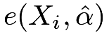
    obtain the fitted values of the propensity scores e(X_{i},\hat{\alpha}) and then obtain the fitted values of the odds o(X_{i},\hat{\alpha})=e(X_{i},\hat{\alpha})/(1-e(X_{i},\hat{\alpha}));

  3. 2.

    obtain the fitted values of the outcome mean under control \mu_{0}(X_{i},\hat{\beta}_{0});

  4. 3.

    construct the doubly robust estimator: \hat{\tau}_{\textsc{T}}^{\textup{dr}}=\hat{\bar{Y}}(1)-\hat{\mu}_{0\textsc{T}}^{\textup{dr}}, where
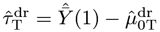
    \hat{\mu}_{0\textsc{T}}^{\textup{dr}}=\frac{1}{n_{1}}\sum_{i=1}^{n}\left[o(X_{i},\hat{\alpha})(1-Z_{i})\{Y_{i}-\mu_{0}(X_{i},\hat{\beta}_{0})\}+Z_{i}\mu_{0}(X_{i},\hat{\beta}_{0})\right].

By Definition 13.1, we can rewrite \hat{\tau}_{\textsc{T}}^{\textup{dr}} as

e(X_{i},\hat{\alpha})=\hat{\tau}_{\textsc{T}}^{\textup{reg}}-\frac{1}{n_{1}}\sum_{i=1}^{n}o(X_{i},\hat{\alpha})(1-Z_{i})\{Y_{i}-\mu_{0}(X_{i},\hat{\beta}_{0})\}

or

e(X_{i},\hat{\alpha})=\hat{\tau}_{\textsc{T}}^{\textup{ht}}-\frac{1}{n_{1}}\sum_{i=1}^{n}\{o(X_{i},\hat{\alpha})(1-Z_{i})+Z_{i}\}\mu_{0}(X_{i},\hat{\beta}_{0}).

Similar to the discussion of \hat{\tau}^{\textup{dr}}, we can estimate the variance of \hat{\tau}_{\textsc{T}}^{\textup{dr}} via the bootstrap by resampling from (Z_{i},X_{i},Y_{i})_{i=1}^{n}. Hahn, (1998), Mercatanti and Li, (2014), Shinozaki and Matsuyama, (2015) and Yang and Ding, 2018b () are references on the estimation of \tau_{\textsc{T}}.

69 An example

The following R function implements two outcome regression estimators, two IPW estimators, and the doubly robust estimator for \tau_{\textsc{T}}. To avoid extreme estimated propensity scores, we can also truncate them from the above.

ATT.est = function(z, y, x, out.family = gaussian, Utruncps = 1)
{
## sample size
nn = length(z)
nn1 = sum(z)
## fitted propensity score
pscore = glm(z ~ x, family = binomial)$fitted.values
pscore = pmin(Utruncps, pscore)
odds = pscore/(1 - pscore)
## fitted potential outcomes
outcome0 = glm(y ~ x, weights = (1 - z),
family = out.family)$fitted.values
## outcome regression estimator
ace.reg0 = lm(y ~ z + x)$coef[2]
ace.reg = mean(y[z==1]) - mean(outcome0[z==1])
## propensity score weighting estimator
ace.ipw0 = mean(y[z==1]) -
mean(odds*(1 - z)*y)*nn/nn1
ace.ipw = mean(y[z==1]) -
mean(odds*(1 - z)*y)/mean(odds*(1 - z))
## doubly robust estimator
res0 = y - outcome0
ace.dr = ace.reg - mean(odds*(1 - z)*res0)*nn/nn1
return(c(ace.reg0, ace.reg, ace.ipw0, ace.ipw, ace.dr))
}

The following R function further implements the bootstrap variance estimators.

OS_ATT = function(z, y, x, n.boot = 10^2,
out.family = gaussian, Utruncps = 1)
{
point.est = ATT.est(z, y, x, out.family, Utruncps)
## nonparametric bootstrap
n = length(z)
x = as.matrix(x)
boot.est = replicate(n.boot, {
id.boot = sample(1:n, n, replace = TRUE)
ATT.est(z[id.boot], y[id.boot], x[id.boot, ],
out.family, Utruncps)
})
boot.se = apply(boot.est, 1, sd)
res = rbind(point.est, boot.se)
rownames(res) = c("est", "se")
colnames(res) = c("reg0", "reg", "HT", "Hajek", "DR")
return(res)
}

Now we re-analyze the data in Example 10.3 to estimate \tau_{\textsc{T}}. We obtain

reg0 reg HT Hajek DR
est 0.061 -0.351 -1.992 -0.351 -0.187
se 0.227 0.258 0.705 0.328 0.287

without truncating the estimated propensity scores, and

reg0 reg HT Hajek DR
est 0.061 -0.351 -0.597 -0.192 -0.230
se 0.223 0.255 0.579 0.302 0.276

by truncating the estimated propensity scores from the above at 0.9. The HT estimator is sensitive to the truncation as expected. The regression estimator in Example 13.1 is quite different from other estimators. It imposes an unnecessary assumption that the regression functions in the treatment and control group share the same coefficient of X. The regression estimator in Example 13.2 is much closer to the Hajek and doubly robust estimators. The estimates above are slightly different from those in Section 64.3, suggesting the existence of treatment effect heterogeneity across \tau_{\textsc{T}} and \tau.

70 Other estimands

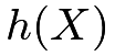
Li et al., 2018a () gave a unified discussion of the causal estimands in observational studies. Starting from the conditional average causal effect \tau(X), they proposed a general class of estimands
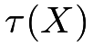
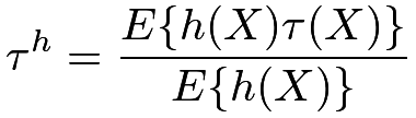
\tau^{h}=\frac{E\{h(X)\tau(X)\}}{E\{h(X)\}}

indexed by a weighting function h(X) with E\{h(X)\}\neq 0. The normalization in the denominator is to ensure that a constant causal effect \tau(X)=\tau averages to the same \tau.
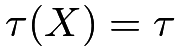
Under ignorability,

\tau^{h}=\frac{E[h(X)\{\mu_{1}(X)-\mu_{0}(X)\}]}{E\{h(X)\}}

which motivates the outcome regression estimator

\hat{\tau}^{h}=\frac{\sum_{i=1}^{n}h(X_{i})\{\hat{\mu}_{1}(X_{i})-\hat{\mu}_{0}(X_{i})\}}{\sum_{i=1}^{n}h(X_{i})}.

Moreover, we can show that \tau^{h} has the following weighting form:

Theorem 13.4

Under the ignorability and overlap assumption, we have

\tau^{h}=E\left\{\frac{ZYh(X)}{e(X)}-\frac{(1-Z)Yh(X)}{1-e(X)}\right\}/E\{h(X)\}.

The proof of Theorem 13.4 is similar to those of Theorems 11.2 and 13.2 which is relegated to Problem 13.9. Based on Theorem 13.4, we can construct the corresponding IPW estimator for \tau^{h}.

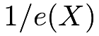
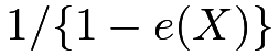
By Theorem 13.4, each unit is associated with the weight due to the definition of the estimand as well as the weight due to the inverse of the propensity score. Finally, the treated units are weighted by h(X)/e(X) and the control units are weighted by h(X)/\{1-e(X)\}. Li et al., 2018a (, Table 1) summarized several estimands, and I present a part of it below:
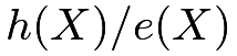

population h(X) estimand weights
combined 1 \tau 1/e(X) and 1/\{1-e(X)\}
treated e(X) \tau_{\textsc{T}} 1 and e(X)/\{1-e(X)\}
control 1-e(X) \tau_{\textsc{C}} \{1-e(X)\}/e(X) and 1
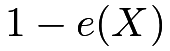
overlap e(X)\{1-e(X)\} \tau_{\textsc{O}} 1-e(X) and e(X)

The overlap population and the corresponding estimand

\tau_{\textsc{O}}=\frac{E\left[e(X)\{1-e(X)\}\tau(X)\right]}{E\left[e(X)\{1-e(X)\}\right]}

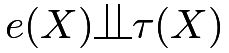
is new to us. This estimand has the largest weight for units with e(X)=1/2 and down weights the units with extreme propensity scores. A nice feature of this estimand is that its IPW estimator is stable without the possibly extremely small values of e(X) and 1-e(X) in the denominator. If e(X)\ind \tau(X) including the special case of \tau(X)=\tau, the parameter \tau_{\textsc{O}} reduces to \tau. In general, however, the estimand \tau_{\textsc{O}} may cause controversy because it changes the initial population and depends on the propensity score which may be misspecified in practice. Li et al., 2018a () and Li et al., (2019) gave some justifications and numerical evidence. This estimand will appear again in Chapter 14.

We can also construct the doubly robust estimator for \tau^{h}. I relegate the details to Problem 13.10.

71 Homework Problems

13.1 Comparing \tau_{\textsc{T}},\tau_{\textsc{C}}, and \tau
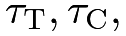
Assume Z\ind \{Y(1),Y(0)\}\mid X. Recall e(X)=\textup{pr}(Z=1\mid X) is the propensity score, e=\textup{pr}(Z=1) is the marginal probability of the treatment, and \tau(X)=E\{Y(1)-Y(0)\mid X\} is the CATE. Show that

\tau_{\textsc{T}}-\tau=\frac{\textup{cov}\{e(X),\tau(X)\}}{e},\quad\tau_{\textsc{C}}-\tau=-\frac{\textup{cov}\{e(X),\tau(X)\}}{1-e}.

Remark: The results above also imply that \tau_{\textsc{T}}-\tau_{\textsc{C}}=\textup{cov}\{e(X),\tau(X)\}/\{e(1-e)\}. So the differences among \tau_{\textsc{T}},\tau_{\textsc{C}},\tau depend on the covariance between the propensity score and CATE. When e(X) and \tau(X) are uncorrelated, their differences are 0.

13.2 An algebraic fact about a regression estimator for \tau_{\textsc{T}}

This problem provides more details for Example 13.2.

Show that if we center the covariates by X_{i}-\hat{\bar{X}}(1) for all units, then \hat{\tau}_{\textsc{T}} equals the coefficient of Z in the OLS fit of the outcome on the intercept, the treatment, covariates, and their interactions.

13.3 Simulation for the average causal effect on the treated units

Chapter 12 ran some simulation studies for \tau. Run similar simulation studies for \tau_{\textsc{T}} with either correct or incorrect propensity score or outcome models.

You can choose different model parameters, a larger number of simulation settings, and a larger number of bootstrap replicates. Report your findings, including at least the bias, variance, and variance estimator via the bootstrap. You can also report other properties of the estimators, for example, the asymptotic Normality and the coverage rates of the confidence intervals.

13.4 An alternative form of the doubly robust estimator for \tau_{\textsc{T}}

Motivated by (73), we have an alternative form of doubly robust estimator for E\{Y(0)\mid Z=1\}:

\tilde{\mu}_{0\textsc{T}}^{\text{dr2}}=\frac{E\left[o(X,\alpha)(1-Z)\{Y-\mu_{0}(X,\beta_{0})\}\right]}{E\left[o(X,\alpha)(1-Z)\right]}+E\{Z\mu_{0}(X,\beta_{0})\}/e.

Show that under Assumption 13.1, \tilde{\mu}_{0\textsc{T}}^{\text{dr2}}=E\{Y(0)\mid Z=1\} if either e(X,\alpha)=e(X) or \mu_{0}(X,\beta_{0})=\mu_{0}(X). Give the sample analog of the doubly robust estimator for \tau_{\textsc{T}}.

13.5 Average causal effect on the control units

Prove the identification formulas for \tau_{\textsc{C}}, analogous to (70) and (72). Propose the doubly robust estimator for \tau_{\textsc{C}}.

13.6 Estimating individual effect and conditional average causal effect

Assume that \{Z_{i},X_{i},Y_{i}(1),Y_{i}(0)\}_{i=1}^{n}\stackrel{{\scriptstyle\textup{IID}}}{{\sim}}\{Z,X,Y(1),Y(0)\}. The individual effect is \tau_{i}=Y_{i}(1)-Y_{i}(0) and the conditional average causal effect is \tau(X_{i})=E\{Y_{i}(1)-Y_{i}(0)\mid X_{i}\}. Since we will discuss the individual effect, we do not drop the subscript i since \tau means the average causal effect, not the population version of Y(1)-Y(0).


  1. 1.

    Under randomization with Z_{i}\ind \{Y_{i}(1),Y_{i}(0)\} and e=\textup{pr}(Z_{i}=1), show that

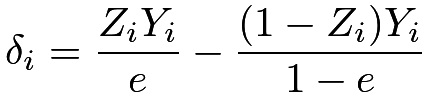
    \delta_{i}=\frac{Z_{i}Y_{i}}{e}-\frac{(1-Z_{i})Y_{i}}{1-e}

    is an unbiased predictor of the individual effect in the sense that

    E(\delta_{i}-\tau_{i})=0\quad(i=1,\ldots,n).

    Further show that E(\delta_{i})=\tau for all i=1,\ldots,n.

  2. 2.

    Under ignorability with Z_{i}\ind \{Y_{i}(1),Y_{i}(0)\}\mid X_{i} and e(X_{i})=\textup{pr}(Z_{i}=1\mid X_{i}), show that

    \delta_{i}=\frac{Z_{i}Y_{i}}{e(X_{i})}-\frac{(1-Z_{i})Y_{i}}{1-e(X_{i})}

    is an unbiased predictor of the individual effect and the conditional average causal effect in the sense that

    E(\delta_{i}-\tau_{i})=0,\quad E\{\delta_{i}-\tau(X_{i})\}=0,\quad(i=1,\ldots,n).

    Further show that E(\delta_{i})=\tau for all i=1,\ldots,n.

13.7 General estimand and (\tau_{\textsc{T}},\tau_{\textsc{C}})

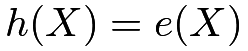
Assume unconfoundedness. Show that \tau^{h}=\tau_{\textsc{T}} if h(X)=e(X), and \tau^{h}=\tau_{\textsc{C}} if h(X)=1-e(X).

13.8 More on \tau_{\textsc{O}}

Show that

\tau_{\textsc{O}}=\frac{E[\{1-e(X)\}\tau(X)\mid Z=1]}{E\{1-e(X)\mid Z=1\}}=\frac{E\{e(X)\tau(X)\mid Z=0\}}{E\{e(X)\mid Z=0\}}.
13.9 IPW for the general estimand

Prove Theorem 13.4.

13.10 Doubly robust estimation for general estimand

For a given h(X), we have the following formulas for constructing the doubly robust estimator for \tau^{h}:

\displaystyle\tilde{\mu}_{1}^{h,\textup{dr}} \displaystyle= \displaystyle E\left[\frac{Zh(X)\{Y-\mu_{1}(X,\beta_{1})\}}{e(X,\alpha)}+h(X)\mu_{1}(X,\beta_{1})\right],
\displaystyle\tilde{\mu}_{0}^{h,\textup{dr}} \displaystyle= \displaystyle E\left[\frac{(1-Z)h(X)\{Y-\mu_{0}(X,\beta_{0})\}}{1-e(X,\alpha)}+h(X)\mu_{0}(X,\beta_{0})\right].

Show that under ignorability and overlap,

  1. 1.

    if either e(X,\alpha)=e(X) or \mu_{1}(X,\beta_{1})=\mu_{1}(X), then \tilde{\mu}_{1}^{h,\textup{dr}}=E\{h(X)Y(1)\};

  2. 2.

    if either e(X,\alpha)=e(X) or \mu_{0}(X,\beta_{0})=\mu_{0}(X), then \tilde{\mu}_{0}^{h,\textup{dr}}=E\{h(X)Y(0)\};

  3. 3.

    if either e(X,\alpha)=e(X) or \{\mu_{1}(X,\beta_{1})=\mu_{1}(X),\mu_{0}(X,\beta_{0})=\mu_{0}(X)\}, then

    \frac{\tilde{\mu}_{1}^{h,\textup{dr}}-\tilde{\mu}_{0}^{h,\textup{dr}}}{E\{h(X)\}}=\tau^{h}.

Remark: Tao and Fu, (2019) proved the above results. However, they hold only for a given h(X). The most interesting cases of \tau_{\textsc{T}},\tau_{\textsc{C}} and \tau_{\textsc{O}} all have weight depending on the propensity score e(X), which must be estimated in the first place. The above formulas do not apply to constructing the doubly robust estimators for \tau_{\textsc{T}} and \tau_{\textsc{C}}; there does not exist a doubly robust estimator for \tau_{\textsc{O}}.

13.11 Analyzing a dataset from the Karolinska Institute

Revisit Problem 12.5. Estimate \tau_{\textsc{T}} based on the methods introduced in this Chapter.

13.12 Recommended reading

Shinozaki and Matsuyama, (2015) focused on \tau_{\textsc{T}}, and Li et al., 2018a () discussed general \tau^{h}.

本书:A First Course in Causal Inference,作者 Peng Ding。原文:arXiv:2305.18793v2,按 CC BY 4.0 许可发布。本站(yuanens.com)把 arXiv 网页版改成分章的纯 HTML,把公式渲染成图片,方便在 Kindle 等电子书阅读器上看,内容没有改动。转换难免有错,以原文为准。本站与作者和出版社无关。