Chapter 22 Disentangle Mixture Distributions and Instrumental Variable Inequalities

The IV model in Chapter 21 imposes Assumptions 21.1–21.3:

  1. 1.

    Z\ind \{D(1),D(0),Y(1),Y(0)\};

  2. 2.

    \textup{pr}(U=\textup{d})=0;

  3. 3.

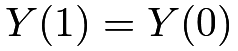
    Y(1)=Y(0) for U=\textup{a} or n.

Table 9 summarizes the observed groups and the corresponding latent groups under the monotonicity assumption.

Table 9: Observed groups and latent groups under Assumption 21.2
Z D D(1) latent groups
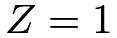
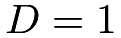
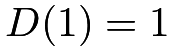
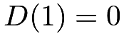
Z=1 D=1 D(1)=1 U=\textup{c} or a
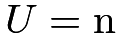
Z=1 D=0 D(1)=0 U=\textup{n}
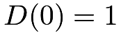
Z=0 D=1 D(0)=1 U=\textup{a}
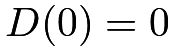
Z=0 D=0 D(0)=0 U=\textup{c} or n

Interestingly, Assumptions 21.1–21.3 together have some testable implications. Balke and Pearl, (1997) called them the instrumental variable inequalities. This chapter will give an intuitive derivation of a special case of these inequalities. The proof is a direct consequence of identifying the means of the potential outcomes for all latent groups defined by U.

110 Disentangle Mixture Distributions

We summarize the main results in Theorem 22.1 below. Define

\pi_{u}=\textup{pr}(U=u)\quad\quad(u=\textup{a},\textup{n},\textup{c})

as the proportion of type U=u, and

\mu_{zu}=E\{Y(z)\mid U=u\}\quad\quad(z=0,1;u=\textup{a},\textup{n},\textup{c}).

as the mean of the potential outcome Y(z) for type U=u. Exclusion restriction implies that \mu_{1\textup{n}}=\mu_{0\textup{n}} and \mu_{1\textup{a}}=\mu_{0\textup{a}}. Let \mu_{\textup{n}} and \mu_{\textup{a}} denote them, respectively.

Theorem 22.1

Under Assumptions 21.1–21.3, we can identify the proportions of the latent types by

\displaystyle\pi_{\textup{n}} \displaystyle= \displaystyle\textup{pr}(D=0\mid Z=1),
\displaystyle\pi_{\textup{a}} \displaystyle= \displaystyle\textup{pr}(D=1\mid Z=0),
\displaystyle\pi_{\textup{c}} \displaystyle= \displaystyle E(D\mid Z=1)-E(D\mid Z=0),

and the type-specific means of the potential outcomes by

\displaystyle\mu_{\textup{n}} \displaystyle= \displaystyle E(Y\mid Z=1,D=0),
\displaystyle\mu_{\textup{a}} \displaystyle= \displaystyle E(Y\mid Z=0,D=1),
\displaystyle\mu_{1\textup{c}} \displaystyle= \displaystyle\pi_{\textup{c}}^{-1}\left\{E(DY\mid Z=1)-E(DY\mid Z=0)\right\},
\displaystyle\mu_{0\textup{c}} \displaystyle= \displaystyle\pi_{\textup{c}}^{-1}\big[E\{(1-D)Y\mid Z=0\}-E\{(1-D)Y\mid Z=1\}\big].

Proof of Theorem 22.1: Part I: We first identify the proportions of the latent compliance types. We can identify the proportion of the never takers by

\displaystyle\textup{pr}(D=0\mid Z=1) \displaystyle= \displaystyle\textup{pr}(U=\textup{n}\mid Z=1)
\displaystyle= \displaystyle\textup{pr}(U=\textup{n})
\displaystyle= \displaystyle\pi_{\textup{n}},

and the proportion of the always takers by

\displaystyle\textup{pr}(D=1\mid Z=0) \displaystyle= \displaystyle\textup{pr}(U=\textup{a}\mid Z=0)
\displaystyle= \displaystyle\textup{pr}(U=\textup{a})=\pi_{\textup{a}}.

Therefore, the proportion of compliers is

\displaystyle\pi_{\textup{c}} \displaystyle= \displaystyle\textup{pr}(U=\textup{c})
\displaystyle= \displaystyle 1-\pi_{\textup{n}}-\pi_{\textup{a}}
\displaystyle= \displaystyle 1-\textup{pr}(D=0\mid Z=1)-\textup{pr}(D=1\mid Z=0)
\displaystyle= \displaystyle E(D\mid Z=1)-E(D\mid Z=0)
\displaystyle= \displaystyle\tau_{D},

which is coherent with our previous discussion. Although we do not know individual latent compliance types for all units, we can identify the proportions of never-takers, always-takers, and compliers.

Part II: We then identify the means of the potential outcomes within latent compliance types. The observed group (Z=1,D=0) only has never takers, so

E(Y\mid Z=1,D=0)=E\{Y(1)\mid Z=1,U=\textup{n}\}=E\{Y(1)\mid U=\textup{n}\}=\mu_{\textup{n}}.

The observed group (Z=0,D=1) only has always takers, so

E(Y\mid Z=0,D=1)=E\{Y(0)\mid Z=0,U=\textup{a}\}=E\{Y(0)\mid U=\textup{a}\}=\mu_{\textup{a}}.

The observed group (Z=1,D=1) has both compliers and always takers, so

\displaystyle E(Y\mid Z=1,D=1) \displaystyle= \displaystyle E\{Y(1)\mid Z=1,D(1)=1\}
\displaystyle= \displaystyle E\{Y(1)\mid D(1)=1\}
\displaystyle= \displaystyle\textup{pr}\{D(0)=1\mid D(1)=1\}E\{Y(1)\mid D(1)=1,D(0)=1\}
\displaystyle+\textup{pr}\{D(0)=0\mid D(1)=1\}E\{Y(1)\mid D(1)=1,D(0)=0\}
\displaystyle= \displaystyle\frac{\pi_{\textup{c}}}{\pi_{\textup{c}}+\pi_{\textup{a}}}\mu_{1\textup{c}}+\frac{\pi_{\textup{a}}}{\pi_{\textup{c}}+\pi_{\textup{a}}}\mu_{\textup{a}}.

Solve the linear equation above to obtain

\displaystyle\mu_{1\textup{c}} \displaystyle= \displaystyle\pi_{\textup{c}}^{-1}\left\{(\pi_{\textup{c}}+\pi_{\textup{a}})E(Y\mid Z=1,D=1)-\pi_{\textup{a}}E(Y\mid Z=0,D=1)\right\}
\displaystyle= \displaystyle\pi_{\textup{c}}^{-1}\left\{\textup{pr}(D=1\mid Z=1)E(Y\mid Z=1,D=1)\right.
\displaystyle\left.\qquad-\textup{pr}(D=1\mid Z=0)E(Y\mid Z=0,D=1)\right\}
\displaystyle= \displaystyle\pi_{\textup{c}}^{-1}\left\{E(DY\mid Z=1)-E(DY\mid Z=0)\right\}.

The observed group (Z=0,D=0) has both compliers and never takers, so

\displaystyle E(Y\mid Z=0,D=0) \displaystyle= \displaystyle E\{Y(0)\mid Z=0,D(0)=0\}
\displaystyle= \displaystyle E\{Y(0)\mid D(0)=0\}
\displaystyle= \displaystyle\textup{pr}\{D(1)=1\mid D(0)=0\}E\{Y(0)\mid D(1)=1,D(0)=0\}
\displaystyle+\textup{pr}\{D(1)=0\mid D(0)=0\}E\{Y(0)\mid D(1)=0,D(0)=0\}
\displaystyle= \displaystyle\frac{\pi_{\textup{c}}}{\pi_{\textup{c}}+\pi_{\textup{n}}}\mu_{0\textup{c}}+\frac{\pi_{\textup{n}}}{\pi_{\textup{c}}+\pi_{\textup{n}}}\mu_{\textup{n}}.

Solve the linear equation above to obtain

\displaystyle\mu_{0\textup{c}} \displaystyle= \displaystyle\pi_{\textup{c}}^{-1}\left\{(\pi_{\textup{c}}+\pi_{\textup{n}})E(Y\mid Z=0,D=0)-\pi_{\textup{n}}E(Y\mid Z=1,D=0)\right\}
\displaystyle= \displaystyle\pi_{\textup{c}}^{-1}\left\{\textup{pr}(D=0\mid Z=0)E(Y\mid Z=0,D=0)\right.
\displaystyle\left.\qquad-\textup{pr}(D=0\mid Z=1)E(Y\mid Z=1,D=0)\right\}
\displaystyle= \displaystyle\pi_{\textup{c}}^{-1}\big[E\{(1-D)Y\mid Z=0\}-E\{(1-D)Y\mid Z=1\}\big].

\square

Based on the formulas of \mu_{1\textup{c}} and \mu_{0\textup{c}} in Theorem 22.1, we can simplify \tau_{\textup{c}}=\mu_{1\textup{c}}-\mu_{0\textup{c}} as

\tau_{\textup{c}}=\{E(Y\mid Z=1)-E(Y\mid Z=0)\}/\pi_{\textup{c}},

which is the same as the formula in Theorem 21.1 before.

Theorem 22.1 focuses on identifying the means of the potential outcomes, \mu_{zu}. Imbens and Rubin, (1997) derived more general identification formulas for the distribution of the potential outcomes; I leave the details to Problem 22.3.

111 Testable implications: Instrumental Variable Inequalities

Is there any additional value of the detour to derive the formula of \tau_{\textup{c}} through Theorem 22.1? The answer is yes. For binary outcome, the following inequalities must be true:

0\leq\mu_{1\textup{c}}\leq 1,\quad 0\leq\mu_{0\textup{c}}\leq 1,

which implies four inequalities

\displaystyle E(DY\mid Z=1)-E(DY\mid Z=0) \displaystyle\geq \displaystyle 0,
\displaystyle E(DY\mid Z=1)-E(DY\mid Z=0) \displaystyle\leq \displaystyle E(D\mid Z=1)-E(D\mid Z=0),
\displaystyle E\{(1-D)Y\mid Z=0\}-E\{(1-D)Y\mid Z=1\} \displaystyle\geq \displaystyle 0,
\displaystyle E\{(1-D)Y\mid Z=0\}-E\{(1-D)Y\mid Z=1\} \displaystyle\leq \displaystyle E(D\mid Z=1)-E(D\mid Z=0).

Rearranging terms, we obtain the following unified inequalities.

Theorem 22.2 (Instrumental Variable Inequalities)

With a binary outcome Y, Assumptions 21.1–21.3 imply

\displaystyle E(Q\mid Z=1)-E(Q\mid Z=0)\geq 0, (104)

where Q=DY,D(1-Y),(D-1)Y and D+Y-DY.

Under the IV assumptions 21.1–21.3, the difference in means for Q=DY,D(1-Y),(D-1)Y and D+Y-DY must all be non-negative. Importantly, these implications only involve the distribution of the observed variables. Rejection of the IV inequalities leads to rejection of the IV assumptions.

Balke and Pearl, (1997) derived more general IV inequalities with and without assuming monotonicity. The proving strategy above is due to Jiang and Ding, (2020) for a slightly more complex setting. Theorem 22.2 states the testable implications only for a binary outcome. Problem 22.4 gives an equivalent form, and Problem 22.5 gives the result for a general outcome.

112 Examples

For a binary outcome, we can estimate all the parameters by the method of moments below.

IVbinary = function(n111, n110, n101, n100,
n011, n010, n001, n000){
n_tr = n111 + n110 + n101 + n100
n_co = n011 + n010 + n001 + n000
n = n_tr + n_co
## proportions of the latent strata
pi_n = (n101 + n100)/n_tr
pi_a = (n011 + n010)/n_co
pi_c = 1 - pi_n - pi_a
## four observed means of the outcomes (Z=z,D=d)
mean_y_11 = n111/(n111 + n110)
mean_y_10 = n101/(n101 + n100)
mean_y_01 = n011/(n011 + n010)
mean_y_00 = n001/(n001 + n000)
## means of the outcomes of two strata
mu_n1 = mean_y_10
mu_a0 = mean_y_01
## ER implies the following two means
mu_n0 = mu_n1
mu_a1 = mu_a0
## stratum (Z=1,D=1) is a mixture of c and a
mu_c1 = ((pi_c + pi_a)*mean_y_11 - pi_a*mu_a1)/pi_c
## stratum (Z=0,D=0) is a mixture of c and n
mu_c0 = ((pi_c + pi_n)*mean_y_00 - pi_n*mu_n0)/pi_c
## identifiable quantities from the observed data
list(pi_c = pi_c,
pi_n = pi_n,
pi_a = pi_a,
mu_c1= mu_c1,
mu_c0= mu_c0,
mu_n1= mu_n1,
mu_n0= mu_n0,
mu_a1= mu_a1,
mu_a0= mu_a0,
tau_c= mu_c1 - mu_c0)
}

We then re-visit two canonical examples with binary data.

Example 22.1

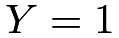
Investigators et al., (2014) assess the effectiveness of the emergency endovascular versus the open surgical repair strategies for patients with a clinical diagnosis of ruptured aortic aneurism. Patients are randomized to either the emergency endovascular or the open repair strategy. The primary outcome is the survival status after 30 days. Let Z be the treatment assigned, with Z=1 for the endovascular strategy and Z=0 for the open repair. Let D be the treatment received. Let Y be the survival status, with Y=1 for dead, and Y=0 for alive. Table 10(a) summarizes the observed data. Using the IVbinary function above, we can obtain the following estimates:

> investigators_analysis = IVbinary(n111 = 107,
+ n110 = 42,
+ n101 = 68,
+ n100 = 42,
+ n011 = 24,
+ n010 = 8,
+ n001 = 131,
+ n000 = 79)
>
> investigators_analysis
$pi_c
[1] 0.4430582
$pi_n
[1] 0.4247104
$pi_a
[1] 0.1322314
$mu_c1
[1] 0.7086064
$mu_c0
[1] 0.6292042
$mu_n1
[1] 0.6181818
$mu_n0
[1] 0.6181818
$mu_a1
[1] 0.75
$mu_a0
[1] 0.75
$tau_c
[1] 0.07940223

There is no evidence of violating the IV assumptions.

Example 22.2

In Hirano et al., (2000), physicians are randomly selected to receive a letter encouraging them to inoculate patients at risk for flu. The treatment is the actual flu shot, and the outcome is an indicator of flu-related hospital visits. However, some patients do not comply with their assignments. Let Z_{i} be the indicator of encouragement to receive the flu shot, with Z=1 if the physician receives the encouragement letter, and Z=0 otherwise. Let D be the treatment received. Let Y be the outcome, with Y=0 if for a flu-related hospitalization during the winter, and Y=1 otherwise. See Problem 21.7 for more details of the data. Table 10(b) summarizes the observed data. Using the IVbinary function above, we can obtain the following estimates:

> flu_analysis = IVbinary(n111 = 31,
+ n110 = 422,
+ n101 = 84,
+ n100 = 935,
+ n011 = 30,
+ n010 = 233,
+ n001 = 99,
+ n000 = 1027)
> flu_analysis
$pi_c
[1] 0.1183997
$pi_n
[1] 0.6922554
$pi_a
[1] 0.1893449
$mu_c1
[1] -0.004548064
$mu_c0
[1] 0.1200094
$mu_n1
[1] 0.08243376
$mu_n0
[1] 0.08243376
$mu_a1
[1] 0.1140684
$mu_a0
[1] 0.1140684
$tau_c
[1] -0.1245575

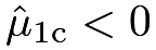
Since \hat{\mu}_{1\textup{c}}<0, there is evidence of violating the IV assumptions.

Table 10: Binary data and IV inequalities
(a) Investigators et al., (2014)’s study
Z=1 Z=0
D=1 D=0 D=1 D=0
Y=1 107 68 24 131
Y=0 42 42 8 79
(b) Hirano et al., (2000)’s study
Z=1 Z=0
D=1 D=0 D=1 D=0
Y=1 31 85 30 99
Y=0 424 944 237 1041

113 Homework problems

22.1 More detailed data analysis

Examples 22.1 and 22.2 ignored the uncertainty in the estimates. Calculate the confidence intervals for the true parameters.

22.2 Risk ratio for compliers

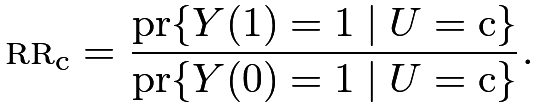
With a binary outcome, we can define the risk ratio for compliers as
\textsc{rr}_{\textup{c}}=\frac{\textup{pr}\{Y(1)=1\mid U=\textup{c}\}}{\textup{pr}\{Y(0)=1\mid U=\textup{c}\}}.

Show that under Assumptions 21.1–21.3, we can identify it by

\textsc{rr}_{\textup{c}}=\frac{E(DY\mid Z=1)-E(DY\mid Z=0)}{E\{(D-1)Y\mid Z=1\}-E\{(D-1)Y\mid Z=0\}}.

Remark: Using Theorem 22.1, we can identify any comparisons between E\{Y(1)\mid U=\textup{c}\} and E\{Y(0)\mid U=\textup{c}\}.

22.3 Disentangle the mixtures: distributional results

This problem extends Theorem 22.1. Define

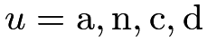
f_{zu}(y)=\textup{pr}\{Y(z)=y\mid U=u\},\quad(z=0,1;u=\textup{a},\textup{n},\textup{c})

as the density of Y(z) for latent stratum U=u, and define

g_{zd}(y)=\textup{pr}(Y=y\mid Z=z,D=d)

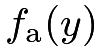
as the density of the outcome within the observed group (Z=z,D=d). Exclusion restriction implies that f_{1\textup{n}}(y)=f_{0\textup{n}}(y) and f_{1\textup{a}}(y)=f_{0\textup{a}}(y). Let f_{\textup{n}}(y) and f_{\textup{a}}(y) denote them, respectively.

Prove Theorem 22.3 below.

Theorem 22.3

Under Assumptions 21.1–21.3, we can identify the type-specific densities of the potential outcomes by

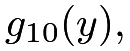
\displaystyle f_{\textup{n}}(y) \displaystyle= \displaystyle g_{10}(y),
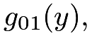
\displaystyle f_{\textup{a}}(y) \displaystyle= \displaystyle g_{01}(y),
\displaystyle f_{1\textup{c}}(y) \displaystyle= \displaystyle\pi_{\textup{c}}^{-1}\{\textup{pr}(D=1\mid Z=1)g_{11}(y)-\textup{pr}(D=1\mid Z=0)g_{01}(y)\},
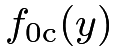
\displaystyle f_{0\textup{c}}(y) \displaystyle= \displaystyle\pi_{\textup{c}}^{-1}\{\textup{pr}(D=0\mid Z=0)g_{00}(y)-\textup{pr}(D=0\mid Z=1)g_{10}(y)\}.
22.4 Alternative form of Theorem 22.2

The inequalities in (104) can be re-written as

\displaystyle\textup{pr}(D=1,Y=y\mid Z=1) \displaystyle\geq \displaystyle\textup{pr}(D=1,Y=y\mid Z=0),
\displaystyle\textup{pr}(D=0,Y=y\mid Z=0) \displaystyle\geq \displaystyle\textup{pr}(D=0,Y=y\mid Z=1)

for both y=0,1.

22.5 IV inequalities for a general outcome

For a general outcome Y, show that Assumptions 21.1–21.3 imply

\displaystyle\textup{pr}(D=1,Y\geq y\mid Z=1) \displaystyle\geq \displaystyle\textup{pr}(D=1,Y\geq y\mid Z=0),
\displaystyle\textup{pr}(D=1,Y<y\mid Z=1) \displaystyle\geq \displaystyle\textup{pr}(D=1,Y<y\mid Z=0),
\displaystyle\textup{pr}(D=0,Y\geq y\mid Z=0) \displaystyle\geq \displaystyle\textup{pr}(D=0,Y\geq y\mid Z=1),
\displaystyle\textup{pr}(D=0,Y<y\mid Z=0) \displaystyle\geq \displaystyle\textup{pr}(D=0,Y<y\mid Z=1)

for all y.

Remark: Imbens and Rubin, (1997) and Kitagawa, (2015) discussed similar results. We can test the first inequality based on an analog of the Kolmogorov–Smirnov statistic:

\text{KS}_{1}=\max_{y}\Big|\frac{\sum_{i=1}^{n}Z_{i}D_{i}1(Y_{i}\leq y)}{\sum_{i=1}^{n}Z_{i}D_{i}}-\frac{\sum_{i=1}^{n}(1-Z_{i})D_{i}1(Y_{i}\leq y)}{\sum_{i=1}^{n}(1-Z_{i})D_{i}}\Big|.
22.6 Example for the IV inequalities

Give an example in which all the IV inequalities hold and another example in which not all the IV inequalities hold. You need to specify the joint distribution of (Z,D,Y) with binary variables.

22.7 Violations of the key assumptions

Theorem 21.1 relies on randomization, monotonicity, and exclusion restriction. The latter two are not testable even in randomized experiments. When they are violated, the IV estimator no longer identifies the CACE. This problem gives two cases below, which are restatements of Propositions 2 and 3 in Angrist et al., (1996). Recall \pi_{u}=\textup{pr}(U=u) and \tau_{u}=E\{Y(1)-Y(0)\mid U=u\} for u=\textup{a},\textup{n},\textup{c},\textup{d}.

Theorem 22.4

(a) Under Assumptions 21.1 and 21.2 without the exclusion restriction, we have

\frac{E(Y\mid Z=1)-E(Y\mid Z=0)}{E(D\mid Z=1)-E(D\mid Z=0)}-\tau_{\textup{c}}=\frac{\pi_{\textup{a}}\tau_{\textup{a}}+\pi_{\textup{n}}\tau_{\textup{n}}}{\pi_{\textup{c}}}.

(b) Under Assumptions 21.1 and 21.3 without the monotonicity, we have

\frac{E(Y\mid Z=1)-E(Y\mid Z=0)}{E(D\mid Z=1)-E(D\mid Z=0)}-\tau_{\textup{c}}=\frac{\pi_{\textup{d}}(\tau_{\textup{c}}+\tau_{\textup{d}})}{\pi_{\textup{c}}-\pi_{\textup{d}}}.

Prove Theorem 22.4.

22.8 Problems of other analyses

In the process of deriving the IV inequalities in Section 110, we disentangled the mixture distributions by identifying the proportions of the latent strata as well as the conditional means of their potential outcomes. These results help to understand the drawbacks of other seemingly reasonable analyses. I review three estimators below and suppose Assumptions 21.1–21.3 hold.

  1. 1.

    The as-treated analysis compares the means of the outcomes among units receiving the treatment and control, yielding

    \tau_{\textsc{at}}=E(Y\mid D=1)-E(Y\mid D=0).

    Show that

    \tau_{\textsc{at}}=\frac{\pi_{\textup{a}}\mu_{\textup{a}}+\textup{pr}(Z=1)\pi_{\textup{c}}\mu_{1\textup{c}}}{\textup{pr}(D=1)}-\frac{\pi_{\textup{n}}\mu_{\textup{n}}+\textup{pr}(Z=0)\pi_{\textup{c}}\mu_{0\textup{c}}}{\textup{pr}(D=0)}.
  2. 2.

    The per-protocol analysis compares the units that comply with the treatment assigned in treatment and control groups, yielding

    \tau_{\textsc{pp}}=E(Y\mid Z=1,D=1)-E(Y\mid Z=0,D=0).

    Show that

    \tau_{\textsc{pp}}=\frac{\pi_{\textup{a}}\mu_{\textup{a}}+\pi_{\textup{c}}\mu_{1\textup{c}}}{\pi_{\textup{a}}+\pi_{\textup{c}}}-\frac{\pi_{\textup{n}}\mu_{\textup{n}}+\pi_{\textup{c}}\mu_{0\textup{c}}}{\pi_{\textup{n}}+\pi_{\textup{c}}}.
  3. 3.

    We may also want to compare the outcomes among units receiving the treatment and control, conditioning on their treatment assignment, yielding

    \displaystyle\tau_{Z=1} \displaystyle= \displaystyle E(Y\mid Z=1,D=1)-E(Y\mid Z=1,D=0),
    \displaystyle\tau_{Z=0} \displaystyle= \displaystyle E(Y\mid Z=0,D=1)-E(Y\mid Z=0,D=0).

    Show that they reduce to

    \tau_{Z=1}=\frac{\pi_{\textup{a}}\mu_{\textup{a}}+\pi_{\textup{c}}\mu_{1\textup{c}}}{\pi_{\textup{a}}+\pi_{\textup{c}}}-\mu_{\textup{n}},\quad\tau_{Z=0}=\mu_{\textup{a}}-\frac{\pi_{\textup{n}}\mu_{\textup{n}}+\pi_{\textup{c}}\mu_{0\textup{c}}}{\pi_{\textup{n}}+\pi_{\textup{c}}}.
22.9 Bounds on the average causal effect on the whole population

Extend the discussion in Section 110 based on the notation in Section 108. With the potential outcome Y(d), define the average causal effect of the treatment received on the outcome as

\delta=E\{Y(d=1)-Y(d=0)\},

and modify the definition of \mu_{zu} as

m_{du}=E\{Y(d)\mid U=u\},\quad(z=0,1;u=\textup{a},\textup{n},\textup{c})

due to the change of the notation. They satisfy

\delta=\sum_{u=\textup{a},\textup{n},\textup{c}}\pi_{u}(m_{1u}-m_{0u}).

Section 110 identifies \pi_{\textup{a}}, \pi_{\textup{n}}, \pi_{\textup{c}}, m_{1\textup{a}}=\mu_{1\textup{a}}, m_{0\textup{n}}=\mu_{0\textup{n}}, m_{1\textup{c}}=\mu_{1\textup{c}} and m_{0\textup{c}}=\mu_{0\textup{c}}. But the data do not contain any information about m_{0\textup{a}} and m_{1\textup{n}}. Therefore, we cannot identify \delta. With a bounded outcome, we can bound \delta.

Theorem 22.5

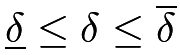
Under Assumptions 21.2–21.4 with a bounded outcome in [\underline{y},\overline{y}], we have \underline{\delta}\leq\delta\leq\overline{\delta}, where

\underline{\delta}=\delta^{\prime}-\overline{y}\textup{pr}(D=1\mid Z=0)+\underline{y}\textup{pr}(D=0\mid Z=1)

and

\overline{\delta}=\delta^{\prime}-\underline{y}\textup{pr}(D=1\mid Z=0)+\overline{y}\textup{pr}(D=0\mid Z=1)

with \delta^{\prime}=E(DY\mid Z=1)-E(Y-DY\mid Z=0).

Prove Theorem 22.5.

Remark: In the special case with a binary outcome, the bounds simplify to

\underline{\delta}=E(DY\mid Z=1)-E(D+Y-DY\mid Z=0)

and

\overline{\delta}=E(DY+1-D\mid Z=1)-E(Y-DY\mid Z=0).
22.10 One-sided noncompliance and statistical inference

Consider a randomized encouragement design where the units assigned to the control have no access to the treatment. For unit i, let Z_{i} be the binary treatment assigned, D_{i} be the binary treatment received, and Y_{i} be the outcome of interest. One-sided noncompliance happens when

Z_{i}=0\Longrightarrow D_{i}=0\quad(i=1,\ldots,n).

Suppose that Assumption 21.1 holds.

  1. [(1)]

  2. 1.

    Does monotonicity Assumption 21.2 hold in this case? How many latent strata defined by \{D_{i}(1),D_{i}(0)\} are there in this problem? How do we identify their proportions by the observed data distribution?

  3. 2.

    State the assumption of exclusion restriction. Under exclusion restriction, show that E\{Y(z)\mid U=u\} can be identified by the observed data distributions. Give the formulas for all possible values of z and u. How do we identify the CACE in this case?

  4. 3.

    If we observe pretreatment covariates X_{i} for all units i, how do we use the covariate information to improve the estimation efficiency of the CACE?

  5. 4.

    Under Assumption 21.1, the exclusion restriction Assumption 21.3 has testable implications, which are the IV inequalities for one-sided noncompliance. State the IV inequalities.

  6. 5.

    Sommer and Zeger, (1991) provided the following dataset:

    Z=1 Z=0
    D=1 D=0 D=1 D=0
    Y=1 9663 2385 0 11514
    Y=0 12 34 0 74

    The treatment assigned Z is whether or not the child was assigned to the vitamin A supplement, the treatment received indicator D is whether or not the child received the vitamin A supplement, and the binary outcome Y is the survival indicator. The original RCT was conducted in Indonesia. Re-analyze the data.

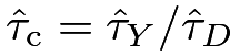
Remark: Bloom, (1984) first discussed one-sided noncompliance and proposed the estimator \hat{\tau}_{\textup{c}}=\hat{\tau}_{Y}/\hat{\tau}_{D}, which is sometimes called the Bloom estimator. Bloom, (1984)’s notation is different from this chapter.
22.11 One-sided noncompliance with partial adherence

Sanders and Karim, (2021, Table 3) reported the following data from an RCT aiming to estimate the efficacy of smoking cessation interventions among individuals with psychotic disorders.

group assigned treatment received group size # positive outcomes
Control None 151 25
Treatment None 35 7
Treatment Partial 42 17
Treatment Full 70 40

Three tiers of treatment received are defined as follows: “full” treatment corresponds to attending all 8 treatment sessions, “partial” corresponds to attending 5 to 7 sessions, and “none” corresponds to <5 sessions. The outcome is defined as the binary indicator of smoking reduction of 50\% or greater relative to baseline, measured at three months.

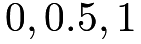
In this problem, the treatment assignment Z is binary but the treatment received D takes three values 0,0.5,1 for “none”, “partial”, and “full.” The three-leveled D causes complications, but it can only be 0 under the control assignment. How many latent strata U=\{D(1),D(0)\} do we have in this problem? Can we identify their proportions?

How do we extend the exclusion restriction to this problem? What can be the causal effects of interest? Can we identify them?

Analyze the data based on the questions above.

22.12 Recommended reading

Balke and Pearl, (1997) derived more general IV inequalities.

本书:A First Course in Causal Inference,作者 Peng Ding。原文:arXiv:2305.18793v2,按 CC BY 4.0 许可发布。本站(yuanens.com)把 arXiv 网页版改成分章的纯 HTML,把公式渲染成图片,方便在 Kindle 等电子书阅读器上看,内容没有改动。转换难免有错,以原文为准。本站与作者和出版社无关。